Download
1 / 28
320 likes | 583 Views
Symbolic – Numeric Algebra in Geodesy. R. Lewis, B. Paláncz, P. Zaletnyik, J. Awange. Geodesy and Surveying. Geodesy and Surveying are concerned with measuring the Earth on different scales.

E N D
Symbolic – Numeric Algebra in Geodesy R. Lewis, B. Paláncz, P. Zaletnyik, J. Awange
Geodesy and Surveying • Geodesy and Surveying are concerned with measuring the Earth on different scales. • Variables such as distances, angles and height differences are measured and other geometrical variables (i. e. coordinates of location) are derived from these measurements. • Many geodetic problems can be represented as systems of multivariable polynomials.
GPS Positioning (GPS Ranging) In GPS Positioning pseudo distances are measured between a GPS receiver and minimum 4 GPS satellites to calculate the position of the receiver (X,Y,Z) and the receiver’ clock bias (T). For each satellites: where ai, bi, ci are the coordinates of the satellites and Pi the measured distances.
3D Helmert similarity transformation In geodesy is a frequent task to calculate the coordinates of points from one to another different coordinate system. In the 7-parameter similarity transformation 3 translations, 3 rotations and 1 scale parameter are used. where R is the rotation matrix, m is the scale parameter and X0, Y0, Z0 are the 3 translation parameters.
Solving Algebraic Computational Problems in Geodesy The book of J.L. Awange and E.W. Grafarend can be considered as a milestone in this research area. The main algebraic methods they applied: • Groebner Basis • Resultants (Sylvester, Macaulay and Sturmfels’ Formulations) • Gauss-Jacobi combinatorial solution 2005
Improvement of models and methods • Geodesy needs more precise measurements, more precise computations with more general and enhanced models. • Computational algebra provides more effective algorithms and methods to carry out these computations.
3D affine transformation The 3D affine transformation is the generalization of the 3D Helmert transformation, using 3 different scale parameters according to the coordinate axes, instead of one. The 9 transformation parameters (3 translation, 3 rotations and 3 scale parameters) should be determined using control points with known coordinates in both coordinate system. where R is the rotation matrix, M the diagonal matrix of the scale parameters and X0, Y0, Z0 are the 3 translation parameters.
Rotation matrix The rotation matrix in general is given by using 3 axial rotation angles (, , - Cardan angles), leading to the next rotation matrix: Instead of the traditional form, the rotation matrix can be expressed with a skew-symmetric matrix (S) also, and this facilitates the symbolic solution of the problem.
Scale parameters In 3D affine transformation 3 scale parameters (m1, m2, m3) are used according to the 3 coordinate axis: In further, instead of the scale parameters (m1, m2, m3), we will use their reciprocals (1, 2, 2) to get more simple equations. introducing:
Using instead of M and we get: The algebraic equations
The 3-point problem As for one point with known coordinates in both coordinate systems3 equations can be written, to determine the 9 parameters of the transformation 3 points are required. In this case the following 9 equations can be written:
Then the system of equation to be solved is, Simplification of the equations We can reduce the equation system by differencingthe equations, and introducing some new variables, the relative coordinates instead of the original ones,
The Dixon – EDF method Explicit symbolic solution can be achieved by employing the accelerated Dixon resultant by the Early Discovery Factors (EDF) algorithm, which was suggested and implemented in the computer algebra system Fermat by Lewis. The basic idea of the Dixon method is to construct a square matrix Mwhose determinantD is a multiple of the resultant. The EDF method is to exploit the observed fact thatD has many factors. In other words, we tryto turn the existence of spurious factors to our advantage. By elementary row and columnmanipulations (Gaussian elimination) we discover probable factors of D and pluck them outof M0=M. Any denominators that form in the matrix are plucked out. This producesa smaller matrix M1 still with polynomial entries, and list of discovered numerators anddenominators.
Using this method one can get theresult in the following form: where i (1) are irreducible polynomials with low degree, but their powers, Kiare very bigpositive integer numbers, so expanding this expression would result into millions of terms! Solution with Dixon – EDF method From our system of equation an univariate polynomial for 1 can be computed by employing the accelerated Dixon resultant by the Early Discovery Factors (Dixon - EDF) algorithm as elimination technique.
Solution with Dixon – EDF method Consequently, we shall consider Ki = 1, for i = 1;…;5. We get five irreducible polynomials (i (1)):
Solution with Dixon – EDF method The factor polynomial providing proper root has degree of two, therefore its solution can be expressed in analytical form (only the positive root is correct, 1). The proper polynomial is: Similarly we can get simple explicit forms for 2 and 3.
Solutions for 1, 2, 3 1 = [X232 y13 z13 + y13 Y232 z13 + X132 y23 z23 + Y132 y23 z23 + y23 Z132 z23 - X13 X23(y23 z13 + y13 z23) - Y13 Y23(y23 z13 + y13 z23) - y23 z13 Z13 Z23 - y13 Z13 z23 Z23 + y13 z13 Z232)]1/2 / [(x23 y13 - x13 y23) (x23 z13 - x13 z23)]1/2 2 = [-X132 x23 z23 + X13 X23(x23 z13 + x13 z23) + x23(Y13 Y23 z13 - Y132 z23 - Z132 z23 + z13 Z13 Z23) - x13(X232 z13 + Y232 z13 - Y13 Y23 z23 - Z13 z23 Z23 + z13 Z232))]1/2 / [-(x23 y13 - x13 y23) (-y23 z13 + y13 z23)]1/2 3 = [X132 x23 y23 - X13 X23(x23 y13 + x13 y23) + x23(Y132 y23 - y13 Y13 Y23 + y23 Z132 - y13 Z13 Z23) + x13(X232 y13 - Y13 y23 Y23 + y13 Y232 - y23 Z13 Z23 + y13 Z232))]1/2 / [(x23 z13 - x13 z23) (y23 z13 - y13 z23)]1/2
Solution for a, b, c Knowing 1, 2, 3 our system of equation will be linear and a, b, c can be determined easily.
Solution for X0, Y0, Z0 Knowing 1, 2, 3 and a, b, c the translation parameters can be determined from the original system of equation: Using the Dixon-EDF method we got fully symbolic solution for all the parameters and using these explicit formulas the parameters can be calculated easily just substituting the coordinates to these formulas.
N-point problem In geodesy normally we have more observations than unknowns, when the solution is determined by minimizing the sum of the deviations squared (Least Squares Method). In this case one possible solution is the before mentioned Gauss-Jacobi combinatorial method. In Hungary there are 1138 national stations with known GPS and local projection coordinates. To determine the parameters of the affine transformation we should have compute about 250 millions combinations, which is unrealistic. Therefore we decided to transform the overdetermined problem into a determined one.
Therefore for N control points we can write 3 times N nonlinear equations. The determined model can be evaluated via partial differentiation: Definition of the N-point problem For one 3D control point (which coordinates are given in both systems), 3 nonlinear equations can be written:
The determined model Using computer algebra manipulations we get a determined model in symbolic form consisting of 9 equations. One of them is:
Numerical solutions of the determined model Unfortunately this multivariate polynomial system of 9 equations with 9 unknowns can not be solved in symbolic form. Local numerical methods like Newton-Raphson or Newton-Krylov generally fail to converge, because of the initial guess values computed from the 3 point solution are wildly different values depending on the constellation of the selected 3 points. Global numerical method like linear homotopy is considered as a good candidate.
Solution with Newton Homotopy Method The homotopy continuation method deforms the known roots of the start system into the roots of the target system. It is a very effective tool to find the roots of polynomial systems. The start values were computed by the 3 point solution, because homotopy solutiontechniqueproved to be very robust to ensure convergency.
Solution with different start values This table illustrates that the values calculated from different triplets can differ significantly depending on their geometrical configurations. The parameters in this table are transformed into their traditional geodetic forms, representing the rotation matrix with three rotation angles (, , ) in seconds, instead of a, b, c, and the deviation of the scale parameters from one (ki=mi–1=1/I-1) in ppm (part per million), instead the inverse scale parameters (1, 2, 3).
Trajectories of the different solutions Solution of the linear homotopy model means the solution of a system of nonlinear ordinary differential equations. Figures above show the trajectories (the homotopy paths) of the variable (parameter) a onthe complex plain, in case of these two different initial values. We have got the same result independently on the initial values.
Comparing the different methods The traditional Newton-Raphson method failed with both initial values, its modification, the Newton-Krylov method had singularity in the first case, and it was slowed down by the increasing number of the iteration ensuring acceptable precision in the second case. Using homotopy we do not need proper initial value, because this method is more robust than local methods, enlarges the domain of convergence and even faster than the traditional Newton’s type methods.