Download

1 / 23
240 likes | 432 Views
Geometry-Based Watermarking of 3D Models. Oliver Benedens. Induction. The idea is to use collections of surfaces as an embedding primitive. A bin is the entity for embedding one bit of watermark data.

E N D
Geometry-BasedWatermarking of3D Models Oliver Benedens
Induction • The idea is to use collections of surfaces as an embedding primitive. • A bin is the entity for embedding one bit of watermark data. • The discrete approximation of the EGI (Extended Gaussian Image) , called an orientation histogram, provides a graphical representation of the described sampling of model normals.
Define a bin • A center normal in 3D space normal and possibly a radius define a bin . The bins can be constructed in a general way by tessellating the unit sphere .
The embedding procedure • (E1) Calculate consistent surface patch normals . • (E2) Sample model normals to bins. • (E3) Apply core watermark embedding algorithm.
Calculating consistent surface normals (E1) • The method depends on consistent surface patch normal directions. • Modelers (or attackers) may produce models with patch normals not pointing in an outward direction; in the extreme, normals point randomly inwards or outwards.
Calculating consistent surface normals (E1) • For each patch cast a ray from the center of mass through the center of the patch and determine angles to both possible normals. • Choose the normal with the greater angle as the surface patch normal. • The triangle points are ordered counterclockwise.
Sample model normals to bins (E2) • NB: the total number of bins :bin centers • : radius (an angle measured in radians; i = 1, …, NB) • Each bini (i = 1, …, NB) is assigned all the model’s normals whose angle difference to the center normal is less than Ri. • BNi: total number of normals sampled to bini. • : the normals sampled in bini.
Core watermark embedding algorithm (E3) the center of mass
Transforming bin normals from a sphere surface representation onto a circle • Normalized 3D vectors BPij (i = 1, …, NB, j = 1, …, BNi) into its 2D coordinate pair pij = (xij, yij) by : h = BCi * BPij , l1 = cos (h), P = BPij - h * BCi(hlies between 0 and 1)
Embedding bit-string S=s1, …,sNB, , i=1, …, NBbe the bit-string to be embedded in model M. Embedding one bit of information in a bin by pushing the center of mass in a certain direction. You’ve successfully coded a “1” bit if the center of mass moves into the marked section of the circle.
Detailed description of the embedding process • function optimizeVertex() to search a vertex’s surroundings for a local cost minimum and itself calls costFunc() to evaluate the costs of certain vertex displacements. • The process also maintains sets containing the original and normal values of triangles as well as their 2D counterparts. main(): d = initial search range for i = 1; i < number of iterations; i++ for each point P in model for j = 1; j < number of refinements; j++ optimizeVertex (P, d) reduce d
optimizeVertex() • optimizeVertex() to find a new local minimum. • The coordinates of point P are updated by replacing P with P’. • the multidimensional downhill simplex lets you explore a given vertex’s neighborhood for a local minimum of costs. initialCosts = costs(P) P’ = multidimensionalDownhillSimplex ( initialCosts, P, d) alter mesh by exchanging P with P’
costFunc (Vertex P) • costFunc() checks for violations of the general constraints. maxCosts=0 if search space exceeded return 2 /* 2 is max value for costs */ for all triangles normals TN adjacent to point P if TN not contained in marked bin if difference (actual TN and original TN) >a return 2 if TN cotained in marked bin if difference (TN and original TN > b) or TN left bin return 2 else c = costs (TN) if (c > maxCosts) maxCosts = c return maxCosts a and b are maximum tolerated normal differences for normals not contained in bins and normals contained in bins, respectively.
costs (Normal N) • The costs c returned to the caller are calculated as follows: with certain weights w1,w2 [0,1] and w1+w2=1
The actual values of variables used in experiments follow • The number of iterations (through the point set) in main() was 3, the number of refinements was 2. • max was 0.3, a= 5 degrees, b = 10 degrees, and d remained constant through all iterations.
Retrieving the watermark Retrieving a watermark requires the reader to know the following a priori information: • The number of bins NB • Their positions (bin center normals) BCi • Their radius Ri • Their original center of mass value comi = (cxi, cyi).
The retrieval algorithm • Calculate consistent surface normal patches (R1). • Transform model into spherical representation and adjust orientation (R2). • Sample model normals to bins (R3). • Core watermark retrieval algorithm (R4).
Core watermark retrieval algorithm (R4) • The bin contents are transformed from 3D to a 2D representation and the center of mass is calculated. • Denote the calculated center of mass values with com’i= (cx’i , cy’i), i = 1, …, NB. • The watermark contents S’ = s’1,…, s’NB, s’i {0,1}, i = 1, …, NBare simply calculated by
The watermarking system wanted primarily to achieve robustness against • Randomization of points • Mesh altering (re-meshing) operations or attacks • Polygon simplification