Download
1 / 54
550 likes | 653 Views
Loss Reserving Using Policy-Level Data. James Guszcza, FCAS, MAAA Jan Lommele, FCAS, MAAA Frank Zizzamia CLRS Las Vegas September, 2004. Agenda. Motivations for Reserving at the Policy Level Outline one possible modeling framework Sample Results. Motivation.

E N D
Loss Reserving Using Policy-Level Data James Guszcza, FCAS, MAAA Jan Lommele, FCAS, MAAA Frank Zizzamia CLRS Las Vegas September, 2004
Agenda • Motivations for Reserving at the Policy Level • Outline one possible modeling framework • Sample Results
Motivation Why do Reserving at the Policy Level?
2 Basic Motivations • Better reserve estimates for a changing book of business • Do triangles “summarize away” important patterns? • Could adding predictive variables help? • More accurate estimate of reserve variability • Summarized data require more sophisticated models to “recover” heterogeneity. • Is a loss triangle a “sufficient statistic” for ultimate losses & variability?
(1) Better Reserve Estimates • Key idea: use predictive variables to supplement loss development patterns • Most reserving approaches analyze summarized loss/claim triangles. • Does not allow the use of covariatesto predict ultimate losses (other than time-indicators). • Actuaries use predictive variables to construct rating plans & underwriting models. • Why not loss reserving too?
Why Use Predictive Variables? • Suppose a company’s book of business has been deteriorating for the past few years. • This decline might not be reflected in a summarized loss development triangle. • However: The resulting change in distributions of certain predictive variables might allow us to refine our ultimate loss estimates.
Examples of Predictive Variables • Claim detail info • Type of claim • Time between claim and reporting • Policy’s historical loss experience • Information about agent who wrote the policy • Exposure • Premium, # vehicles, # buildings/employees… • Other specifics • Policy age, Business/policyholder age, credit…..
More Data Points • Typical reserving projects use claim data summarized to the year/quarter level. • Probably an artifact of the era of pencil-and-paper statistics. • In certain cases important patterns might be “summarized away”. • In the computer age, why restrict ourselves? • More data points less chance of over-fitting the model.
Danger of over-fitting • One well known example • Overdispersed Poisson GLM fit to loss triangle. • Stochastic analog of the chain-ladder • 55 data points • 20 parameters estimated parameters have high standard error. • How do we know the model will generalize well on future development? • Policy-level data: 1000’s of data points
Out-of-Sample Testing • Policy-level dataset has 1,000’s of data points • Rather than 55 data points. • Provides more flexibility for various out-of-sample testing strategies. • Use of holdout samples • Cross-validation • Uses: • Model selection • Model evaluation
(2) Reserve Variability • Variability Components • Process risk • Parameter risk • Model specification risk • Predictive error = process + parameter risk • Both quantifiable • What we will focus on • Reserve variability should also consider model risk. • Harder to quantify
Reserve Variability • Can policy-level data give us a more accurate view of reserve variability? • Process risk: we are not summarizing away variability in the data. • Parameter risk: more data points should lead to less estimation error. • Prediction variance: brute force “bootstrapping” easily combines Process & Parameter variance. • Leaves us more time to focus on model risk.
Disadvantages • Expensive to gather, prepare claim-detail information. • Still more expensive to combine this with policy-level covariates. • More open-ended universe of modeling options (both good and bad). • Requires more analyst time, computer power, and specialist software. • Less interactive than working in Excel.
Modeling Approach Sample Model Design
Philosophy • Provide an example of how reserving might be done at the policy level • To keep things simple: consider a generalization of the chain-ladder • Just one possible model • Analysis is suggestive rather than definitive • No consideration of superimposed inflation • No consideration of calendar year effects • Model risk not estimated • etc…
Notation • Lj = {L12, L24, …, L120} • Losses developed at 12, 24,… months • Developed from policy inception date • PYi = {PY1, PY2, …, PY10 } • Policy Years 1, 2, …, 10 • {Xk}= covariates used to predict losses • Assumption: covariates are measured at or before policy inception
Model Design • Build 9 successive GLM models • Regress L24 on L12; L36 on L24 … etc • Each GLM analogous to a link ratio. • The Lj Lj+1 model is applied to either • Actual values @ j • Predicted values from the Lj-1Ljmodel • Predict Lj+1 using covariates along with Lj.
Model Design • Idea: model each policy’s loss development from period Lj to Lj+1 as a function of a linear combination of several covariates. • Policy-level generalization of the chain-ladder idea. • Consider case where there are no covariates
Model Design • Over-dispersed Poisson GLM: • Log link function • Variance of Lj+1 is proportional to mean • Treat log(Lj) as the offset term • Allows us to model rate of loss development
Using Policy-Level Data • Note: we are using policy-level data. • Therefore the data contains many zeros • Poisson assumption places a point mass at zero • How to handle IBNR • Include dummy variable indicating $0 loss @12 mo • Interact this indicator with other covariates. The model will allocate a piece of the IBNR to each policy with $0 loss as of 12 months.
Data • Policy Year 1991 – 1st quarter 2000 • Workers Comp • 1 record per policy, per year • Each record has multiple loss evaluations • @ 12, 24, …,120 months • “Losses @ j months” means: • j months from the policy inception date. • Losses coded as “missing” where appropriate • e.g., PY 1998 losses at 96 months
Covariates • Historical LR and claim frequency variables • $0 loss @ 12 month indicator • Credit Score • Log premium • Age of Business • New/renewal indicator • Selected policy year dummy variables • Using a PY dummy variable is analogous to leaving that PY out of a link ratio calculation • Use sparingly
Covariates • Interaction terms between covariates and the $0-indicator • Most covariates only used for the 1224 GLM • For other GLMs only use selected PY indicators • These GLMs give very similar results to the chain ladder
Comments • Policy-Level model produces results very close to chain-ladder. • is a proper generalization of the chain-ladder • The model covariates are all statistically significant, have parameters of correct sign. • In this case, the covariates seem to have little influence on the predictions. • Might play more of a role in a book where quality of business changes over time.
Model Evaluation Treat Recent Diagonals as Holdout 10-fold Cross-Validation
Cross-Validation Methodology • Randomly break data into 10 pieces • Fit the 9 GLM models on pieces 1…9 • Apply it to Piece 10 • Therefore Piece 10 is treated as out-of-sample data • Now use pieces 1…8,10 to fit the nine models; apply to piece 9 • Cycle through 8 other cases
Cross-Validation Methodology • Fit 90 GLMs in all • 10 cross-validation iterations • Each involving 9 GLMs • Each of the 10 “predicted” pieces will be a 10x10 matrix consisting entirely of out-of-sample predicted values • Can compare actuals to predicteds on upper half of the matrix • Each cell of the triangle is treated as out-of-sample data
Reserve Variability Using the Bootstrap to estimate the probability distribution of one’s outstanding loss estimate
The Bootstrap • The Statistician Brad Efron proposed a very simple and clever idea for mechanically estimating confidence intervals: The Bootstrap. • The idea is to take multiple resamples of your original dataset. • Compute the statistic of interest on each resample • you thereby estimate the distribution of this statistic!
Motivating Example • Suppose we take 1000 draws from the normal(500,100) distribution • Sample mean ≈ 500 • what we expect • a point estimate of the “true” mean • From theory we know that:
Sampling with Replacement • Draw a data point at random from the data set. • Then throw it back in • Draw a second data point. • Then throw it back in… • Keep going until we’ve got 1000 data points. • You might call this a “pseudo” data set. • This is not merely re-sorting the data. • Some of the original data points will appear more than once; others won’t appear at all.
Sampling with Replacement • In fact, there is a chance of (1-1/1000)1000≈ 1/e ≈ .368 that any one of the original data points won’t appear at all if we sample with replacement 1000 times. any data point is included with Prob ≈ .632 • Intuitively, we treat the original sample as the “true population in the sky”. • Each resample simulates the process of taking a sample from the “true” distribution.
Resampling • Sample with replacement 1000 data points from the original dataset S • Call this S*1 • Now do this 399 more times! • S*1, S*2,…, S*400 • Compute X-bar on each of these 400 samples
The Result • The green bars are a histogram of the sample means of S*1,…, S*400 • The blue curve is a normal distribution with the sample mean and s.d. • The red curve is a kernel density estimate of the distribution underlying the histogram • Intuitively, a smoothed histogram
The Result • The result is an estimate of the distribution of X-bar. • Notice that it is normal with mean≈500 and s.d.≈3.2 • The purely mechanical bootstrapping procedure produces what theory tells us to expect. • Can we use resampling to estimate the distribution of outstanding liabilities?
Bootstrapping Reserves • S = our database of policies • Sample with replacement all policies in S • Call this S*1 • Same size as S • Now do this 199 more times! • S*1, S*2,…, S*200 • Estimate o/s reserves on each sample • Get a distribution of reserve estimates
Bootstrapping Reserves • Compute your favorite reserve estimate on each S*k • These 200 reserve estimates constitute an estimate of the distribution of outstanding losses • Notice that we did this by resampling our original dataset S of policies. • This differs from other analyses which bootstrap the residuals of a model. • Perhaps more theoretically intuitive. • But relies on assumption that your model is correct!
Bootstrapping Results • Standard Deviation ≈ 5% of total o/s losses • 95% confidence interval ≈ (-10%, +10%) • Tighter interval than typically seen in the literature. • Result of not summarizing away variability info?