Download
1 / 70
700 likes | 720 Views
Optical Flow Sensing Theory & Applications Training. Presenter: Paul Lawrence, Sr. Service Engineer. Review of the handouts – (specifications are on the backside of brochure pages). Memory Key Manuals Cheat Sheet This ppt. The Optical Scientific OFS 2000 Flow Meter. CONTROL PANEL.

E N D
Optical Flow SensingTheory & Applications Training Presenter: Paul Lawrence, Sr. Service Engineer
Review of the handouts – (specifications are on the backside of brochure pages) • Memory Key • Manuals • Cheat Sheet • This ppt
The Optical Scientific OFS 2000 Flow Meter CONTROL PANEL INPUT POWER POWER AIRFLOW OUTPUT
Description: Correlation readout Meter Display Magnitude of the time lagged covariance function (ie Correlation or Corr), from the latest scan, is always displayed on the screen and sent to an output. Empirical studies have shown that a correlation value steadily over 100 gives a strong enough waveform shape match for accurate measurements. (i.e It can clearly “see” the eddies and they are traveling in line with the detectors.)
How does the Optical Meter work? RECEIVER TRANSMITTER A BEAM PATH LED B FLOW DEM PREAMP DEM PREAMP AMP ADC Vel Corr A B DIGITAL PROCESSOR COVARANCE PROCESSOR AMP ADC OFS SIGNAL PROCESSOR ELECTRONICS ENCLOSURE RS-232 OUT
Creation of shadows and the ability to “see” eddies of turbulence
Description: Raw data signals Audio waveform of a single gust of air in a duct before the damper was opened Once the flow increases the scintillation in time domain looks like white noise
OFS Digital Processing an actual way the meter does it • Refractive index differences in flow create shadows on the detectors • Patterns create a waveform shape or signature (actual signal detected) • True velocity determined from time it takes signature A to show up in B • It uses the time lagged co-variance function
Review of the history of the technology and milestones in development Discovery & Proof of Principle Paper #1 – 1971 by NOAA
Review of the history of the technology and milestones in development Proof of Principle Paper – 1971 by NOAA
Review of the history of the technology and milestones in development Proof of Principle Paper #1 – highlights - 1971
Review of the history of the technology and milestones in development Proof of Principle Paper #1 – highlights - 1971
Review of the history of the technology and milestones in development Proof of Principle Paper #1 – highlights - 1971
Review of the history of the technology and milestones in development Proof of Principle Paper #1 – highlights - 1971 Equal weighting of the measurement over the pathlength and solving pattern (eddy) decay.
Review of the history of the technology and milestones in development Proof of Principle Paper #2 – 1977 by NOAA Dr. T. Wang went on to found Optical Scientific in 1985, and then acquired this technology and patented it. He is a Fellow of the Optical Society of America (OSA) and a Senior Member of the IEEE.
Review of the history of the technology and milestones in development Proof of Principle Paper #2 – highlights 1977 • Research showed that at shorter pathlengths and stronger turbulence, a laser scintillometer would quickly saturate and no longer “see” the signal. In addition, the calibration and pathlength sensitivity (weighting) would vary with changes in turbulence. • The use of “white light”(non-laser) and larger receiver optics solved this problem and in-addition, a differential signal processing technique was developed to cancel out the effect of vibration and electrical noise. • This opened up the opportunity for short pathlength industrial measurements (smoke and flare stack)
Subsequent Patents given to OSI in 2002 and 2003 for the OFS EXAMPLE
Description: How do we classify the OFS as a meter? BY:Methodology* BY: Installation Style Differential Producers: Orifice, Venturi, Pitot Tube, Etc. Linear Flow Meters: Turbine, Vortex, Magnetic, Ultrasonic, Optical, Positive displacement, Mass flow (Thermal, Coriolis Etc). Insertion Pipe Section Clamp on OFS is a Bolt on, using window barriers. *Reference:Flow Measurement Engin. Handbook, Richard Miller, 1996, 3rd Edition
Description: Low Temperature “lift-off” – need 100o F For Emissions applications (non-flare measurements) it has been shown that at gas temperatures below 100 deg F, the refraction / diffraction phenomena is not strong enough for stable operation (Stable Operation = Correlation values steadily over 100). Add a tracer – a small slip stream of thermal (optical) turbulence
40 30 20 OFS WIND SPEED (M/S) 10 0 0 10 20 30 40 NIST WIND SPEED (M/S) Description: NIST Test: OFS vs. NIST Standard Array Avg.
Description: Actual velocity vs Standardized measurements Tachometer for shadows going by: We have described is the development of a meter that measures the instantaneous average velocity along a line which stretches across the pipe. It works by clocking the speed of optical shadows crossing that line. A kind-of a “tachometer for shadows going by”. It measures is the ACTUAL velocity in feet per second (Afs). If you multiply by the cross sectional area of the pipe you get actual volume in cubic feet per second (Acfs). If you want STANDARDIZED volume, you have to separately measure the temperature and pressure in the pipe and normalize the Acfs reading to standard temperature and pressure, thereby getting standard cubic feet per second (Scfs)
Implications in the real world: Flow is messy The NIST calibration is a great demonstration of the capability of the OFS hardware, BUT it doesn’t mean you can just bolt this meter onto your pipe and expect it to read within 2%, …unless your pipe happens to also be a wind tunnel. Flow in industrial pipes deviates from perfect conditions by ‘influence quantities’* The four major ones are: velocity profile deviations, non-homogenous flow, pulsating flow and cavitation. The Flow Measurement handbook goes on to say: “Velocity profile is probably the most important (and least understood) influence quantity. The effects of swirl…and nonaxis-symetric profiles on a meter’s performance are not only difficult to analyze, but cannot easily be duplicated in the laboratory.”* *Reference: Flow Measurement Engin. Handbook, Richard Miller, 1996, 3rd Edition
Implications in the real world: The well developed profile The OFS meter is used typically in larger pipes (from one foot to 30 feet or more) and in these installations it is rarer to have a well developed flow profile, simply because this doesn’t form until 10 to 20 pipe diameters from a disturbance. If you have a well developed flow profile, Great! But the odds are that you won’t in many applications. *Reference:Flow Measurement Engin. Handbook, Richard Miller, 1996, 3rd Edition
Implications in the real world: - Placing the beam Plane of the bend Here you have a single elbow and the velocity velocity profile coming out of the elbow is skewed and has an uneven structure. If your OFS light beam is in the direction of A , perpendicular to the plane of the bend, then your measurement beam will catch an area that doesn’t vary proportionately with load. If you shoot in the plane of the bend, B it will vary with load. B A *Reference:Flow Measurement Engin. Handbook, Richard Miller, 1996, 3rd Edition
Example of measuring in a single cross-section of the velocity profile
Implications in the real world: - Five rules of Installation #1 Intersect the skewed (and load varying) structure of the velocity profile by locating the beam in the plane of the bend (disturbance). #2 The pipe must be full of flowing gas/air (it only “sees” flowing gas) #3 The flow direction must be the same as the detector alignment (within +/- 20%) #4 Be very careful of being close to control elements like dampers, which create an explosively turbulent environment upstream and downstream, at certain opening positions. #5Be very careful of pipes which carry the shared flow from multiple, undifferentiated, load sources, because then the profile may move sideways in one direction with one of the loads, and in a different direction with the other load.
Review of different real world applications: Stability Linearity Flare applications Combustion Air Loop Close proximity to a damper
Review of different real world applications: Stability Two meters - Nine years without any adjustment
Review of different real world applications: Linearity with known strong cyclonic flow
Review of different real world applications: Flare applications Baseline Zoom fps fps 24 inch line
Review of different real world applications: Combustion Air Loop 3 second response time
Review of different real world applications: Close proximity to a damper and excessive turbulence OFS one diameter away from damper
Review of different real world applications: Very High Temperature
Many Varied Industrial Flow metering applications: • Stacks • Ducts • Combustion Air • After Wet scrubbers • Flare stacks and lines • High Temperature • Cyclonic Flow Problems • Positive or negative pressure • Odd shapes • Tight space and small footprint • On existing angled ports • Very long paths (distances)
A review of the great variation in flow applications that have been tackled by the OFS: ……A Flow meter that can be used in many different applications is a big advantage