Download
1 / 35
350 likes | 637 Views
Costs. APEC 3001 Summer 2007 Readings: Chapter 10 & Appendix in Frank. Objectives. Short Run Production Costs Long Run Production Costs Long Run Production Costs & Industry Structure. Short Run Production Costs Definitions. Total Cost (TC): All costs of production in the short run.

E N D
Costs APEC 3001 Summer 2007 Readings: Chapter 10 & Appendix in Frank
Objectives • Short Run Production Costs • Long Run Production Costs • Long Run Production Costs & Industry Structure
Short Run Production CostsDefinitions • Total Cost (TC): • All costs of production in the short run. • Fixed Cost (FC): • Cost that does not vary with the level of output in the short run. • Variable Cost (VC): • Cost that varies with the level of output in the short run. Important Relationship: TC = VC + FC
Derivation of Short Run Production Costs • Suppose • we have only two inputs labor (L) & capital (K) such that Q = F(K,L). • the price of labor is w & the price of capital is r. • In the short run, some inputs are fixed, say K = K0 such that Q = F(K0,L) = F0(L). • VC = wL = wF0-1(Q) • FC = rK0 • TC = wL + rK0 = wF0-1(Q) + rK0 Important To Remember: TC & VC are functions of Q, not L or K! FC is not a function of Q, L, or K!
Example of Variable, Fixed, & Total Cost Curve Cost TC = wF0-1(Q) + rK0 VC = wF0-1(Q) FC = rK0 Output (Q)
A Numeric Example of TC, VC, & FC • Suppose • we have only two inputs labor (L) & capital (K) such that Q = KL0.5. • the price of labor is w = $15 & the price of capital is r = $25. • In the short run, some inputs are fixed, say K = K0 = 10 such that Q = 10L0.5 and L = Q2/102 = Q2/100. • VC = wL = 15Q2/100 = 0.15Q2 • FC = rK = 2510 = 250 • TC = wL + rK0 = 0.15Q2 + 250 Important To Remember: TC & VC are functions of Q, not L or K! FC is not a function of Q, L, or K!
Short Run Production CostsSome More Definitions • Average Total Cost (ATC): • Total cost divided by the quantity of output, ATC = TC/Q. • Average Fixed Cost (AFC): • Fixed cost divided by the quantity of output, AFC = FC/Q. • Average Variable Cost (AVC): • Variable cost divided by the quantity of output, AVC = VC/Q. • Marginal Cost (MC): • Change in total cost resulting from a one unit increase in output, MC = TC/Q = VC/Q = wF0-1’(Q) where TC, VC, & Q are the change in TC, VC, & Q. Important Relationship: ATC = AVC + AFC Important To Remember: ATC, AVC, & AFC are functions of Q, not L or K!
Graphical Interpretation of ATC, AVC, AFC & MC • ATC is the slope of a line from origin to total cost curve. • AVC is the slope of a line from origin to variable cost curve. • AFC is the slope of a line from origin to fixed cost curve. • MC is the slope of a line tangent to the total & variable cost curves.
Graphical Relationships Costs & Average Costs TC Cost Slope = AFC for Q0 Slope = ATC for Q0 VC Slope = AVC for Q0 FC Q0 Output (Q)
Graphical Relationships Costs & Marginal Costs Cost TC Slope = MC for Q0 Slope = MC for Q0 VC FC Q0 Output (Q)
Relationship Between ATC, AVC, AFC, & MC Cost a: minimum MC b: minimum AVC c: minimum ATC MC AFC is Decreasing ATC c AVC b a AFC Q1 Q2 Q3 Output (Q)
Relationship Between ATC, AVC, AFC, & MC Cost TC a: minimum MC b: minimum AVC c: minimum ATC VC c a b FC Q1 Q2 Q3 Output (Q)
A Numeric Example of ATC, AVC, AFC, & MC • Suppose • we have only two inputs labor (L) & capital (K) such that Q = KL0.5. • the price of labor is w = $15 & the price of capital is r = $25. • In the short run, some inputs are fixed, say K = K0 = 10 such that Q = 10L0.5 and L = Q2/102 = Q2/100. • VC = wL = 15Q2/100 = 0.15Q2 AVC = VC/Q = 0.15Q2/Q = 0.15Q • FC = rK = 2510 = 250 AFC = FC/Q = 250/Q • TC = wL + rK0 = 0.15Q2 + 250 ATC = TC/Q = (0.15Q2 + 250 )/Q = 0.15Q + 250/Q • MC = TC’ = VC’ = 2 0.15Q2-1 = 0.3Q Important To Remember: ATC, AVC, & AFC are functions of Q, not L or K!
A Few More Important Relationships • MC = w/MPL • When MC is at a minimum, MPL is at a maximum. • AVC = wL/Q & APL = Q/L, so AVC = w/APL • When AVC is at a minimum, APL is at a maximum.
Long Run Production Costs • In the long run, there are no fixed costs! • Suppose • there are only two inputs labor (L) & capital (K). • the price of labor is w and the price of capital is r. • Long Run Total Costs (LTC) then equals total expenditures on labor & capital: LTC = wL + rK. • Definition • Isocost Curve: • All combinations of inputs that result in the same cost of production. • If LTC is set constant to say C0, C0 = wL + rK K = C0/r – wL/r. • Equation of a Line • Intercept = C0/r • Slope = -w/r
Graphical Example of Isocost Curve Capital (K) C0/r Slope = -w/r C0/w Labor (L)
Graphical Example of Isocost Map Capital (K) C2/r C2 > C1 > C0 C1/r C0/r Slope = -w/r C0/w C1/w C2/w Labor (L)
Long Run Production Costs • Question: If a firm wants to produce some level of output, say Q0, how much L & K should it use? • Remember • Isoquants tells us the most efficient combinations of inputs for producing some level of output. • So, why not look at our isoquant with our isocost curves?
Example Isocost Map and Isoquant Capital (K) We can efficiently produce Q0 at points like a, b, or c! C2/r How do we choose which point is best? C1/r b C0/r a c Q0 C0/w C1/w C2/w Labor (L)
Important Assumption for Long Run Production Costs • Choose a combination of inputs that minimize costs! • Point a is better than point b or c because costs are lower! • But is there a point that is better than a? • No! To decrease costs below C1 we must reduce L, K, or both, but monotonicity implies that reducing L, K, or both must reduce output below Q0. • What condition holds at point a? • The isocost curve for C1 is just tangent to the isoquant for Q0. • The slope of the isocost curve for C1 equals the slope of the isoquant for Q0: MRTS = w/r.
Intuitive Interpretation of MRTS = w/r • MRTS = MPL/MPK • MRTS = w/r MPL/MPK = w/r MPL/w = MPK/r • MPL/w is the increase in output for an extra $1 spent on L. • MPK/r is the increase in output for an extra $1 spent on K. • Cost are minimized when the increase in output for a $1 spent on L just equals the increase in output for a $1 spent on K. • MRTS > w/r MPL/w > MPK/r • We can reduce costs & produce the same level of output by using more L & less K. • MRTS < w/r MPK/r > MPL/w • We can reduce costs & produce the same level of output by using more K & less L.
Long Run Production CostsAnother Definition • Output Expansion Path: • The locus of tangencies (minimum cost input combinations) traced out by an isocost line of a given slope as it shifts outward into the isoquant map for the production process.
Output Expansion Path Capital (K) C2/r The output expansion path can be used to derive long run costs! C2 > C1 > C0 C1/r C0/r Output Expansion Path c b Q2 > Q1 > Q0 a Q2 Q1 Q0 C0/w C1/w C2/w Labor (L)
Long Run Total Cost Curve Cost LTC c C2 b C1 a C0 Q0 Q1 Q2 Output (Q)
Long Run Production CostsSome More Definitions • Long Run Average Cost (LAC): • Long run cost divided by the quantity of output, LAC = LTC/Q. • Long Run Marginal Cost (LMC): • Change in long run cost resulting from a one unit increase in output, LMC = LTC/Q = LTC’.
Graphical Interpretation of Long Run Average Cost Cost LTC C0 Slope = LAC for Q0 Q0 Output (Q)
Graphical Interpretation of Long Run Marginal Cost Cost LTC Slope = LMC for Q0 C0 Q0 Output (Q)
Long Run Average and Marginal Cost Cost a: minimum LMC b: minimum LAC LMC LAC b a Q0 Q1 Output (Q)
Graphical Interpretation of Long Run Marginal Cost Cost a: minimum LMC LTC b: minimum LAC b a Q0 Q1 Output (Q)
A Numeric Example of ATC, AVC, AFC, & MC • Suppose • we have only two inputs labor (L) & capital (K) such that Q = KL. • the price of labor is w = $10 & the price of capital is r = $40.
Long Run Production Costs & Industry Structure • Long Run Average Costs Can Take A Variety of Shapes • Increasing • Decreasing • Constant • U • The shape of the LAC tells us something about industry structure.
$/Q $/Q $/Q $/Q Output (Q) Output (Q) Output (Q) Output (Q) Types of Long Run Average Cost Decreasing LAC Increasing LAC U-Shaped LAC Constant LAC
Industry Structure & LAC • Increasing LAC • Small Firms Produce At Lowest Average Cost Industry With Lots of Small Firms • Decreasing LAC • A Single Firm Can Produce At Lowest Average Cost Industry With Only One Firm • Natural Monopoly: An industry whose market output is produced at lowest cost when production is concentrated in the hands of a single firm. • Constant LAC • Firm Size Doesn’t Matter At Lowest Average Cost Industry With Lots of Different Firm Sizes • U LAC • A Specific Firm Size Can Produce At Lowest Average Cost Industry With Several Same Size Firms
So, what type of industry is it? • Suppose • we have only two inputs labor (L) & capital (K) such that Q = KL. • the price of labor is w = $10 & the price of capital is r = $40. • Recall From Before: LAC = 40Q-0.5 • LAC’ = -0.540Q-0.5-1 = -20Q-1.5 < 0 • Decreasing Cost
What You Need To Know • Short Run Production Costs • Variable, Fixed, & Total Costs • Average Variable, Fixed, & Total Costs • Marginal Costs • Long Run Production Costs • Long Run Cost, Long Run Average Cost, & Long Run Marginal Cost • Long Run Production Costs & Industry Structure • Increasing, Decreasing, Constant, & U Shaped Average Cost Industries