Download
1 / 15
280 likes | 671 Views
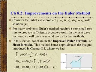
Ch 8.2: Improvements on the Euler Method. Consider the initial value problem y ' = f ( t , y ), y ( t 0 ) = y 0 , with solution ( t ).

E N D
Ch 8.2: Improvements on the Euler Method • Consider the initial value problem y' = f (t, y), y(t0) = y0, with solution (t). • For many problems, Euler’s method requires a very small step size to produce sufficiently accurate results. In the next three sections, we will discuss several more efficient methods. • In this section, we examine the Improved Euler Formula, or Heun formula. This method better approximates the integral introduced in Chapter 8.1, where we had
Improved Euler Method • Consider again the integral equation • Approximating the integrand f (tn, (tn)) with the average of its values at the two endpoints (see graph below), we obtain • Replacing(tn+1) and (tn) by yn+1 andyn, we obtain
Improved Euler Method • Our formula defines yn+1 implicitly, instead of explicitly: • Replacingyn+1 by its value from the Euler formula we obtain the improved Euler formula where fn = f (tn, yn) and tn+1=tn + h.
Error Estimates • The improved Euler formula is • It can be shown that the local truncation error is proportional to h3. This is an improvement over the Euler method, where the local truncation error is proportional to h2. • For a finite interval, it can be shown that the global truncation error is bounded by a constant times h2. Thus the improved Euler method is a second order method, whereas Euler’s method is a first order method. • This greater accuracy comes at expense of more computational work, as it is now necessary to evaluate f(t, y) twice in order to go from tn to tn+1.
Comparison of Euler and Improved Euler Computations • The Euler and improved Euler formulas are given by, respectively, • The improved Euler method requires two evaluations of f at each step, whereas the Euler method requires only one. • This is significant because typically most of the computing time in each step is spent evaluating f. • Thus, for a given step size h, the improved Euler method requires twice as many evaluations of f as the Euler method. • Alternatively, the improved Euler method for step size h requires the same number of evaluations of f as the Euler method with step size h/2.
Trapezoid Rule • The improved Euler formula is • If f(t, y) depends only on t and not on y, then we have which is the trapezoid rule for numerical integration.
Example 1: Improved Euler Method (1 of 3) • For our initial value problem we have • Further, • For h = 0.025, it follows that • Thus
Example 1: Second Step (2 of 3) • For the second step, we have • Also, and • Therefore
Example 1: Numerical Results(3 of 3) • Recall that for a given step size h, the improved Euler formula requires the same number of evaluations of f as the Euler method with step size h/2. • From the table below, we see that the improved Euler method is more efficient, and yields substantially better results or requiring much less total computing effort, or both.
Programming Outline • A computer program for the improved Euler’s method with a uniform step size will have the following structure. • Step 1. Define f (t,y) • Step 2. Input initial values t0 and y0 • Step 3. Input step size h and number of steps n • Step 4. Output t0 and y0 • Step 5. For j from 1 to n do • Step 6. k1 = f (t, y) k2 = f (t + h, y + h*k1) y = y + (h/2)*(k1 + k2) t = t + h • Step 7. Output t and y • Step 8. End
Variation of Step Size (1 of 2) • In Chapter 8.1 we mentioned that adaptive methods adjust the step size as calculations proceed, so as to maintain the local truncation error at roughly a constant level. We outline such a method here. • Suppose that after n steps, we have reached the point (tn, yn). • We next choose an h and then calculate yn+1. • To estimate the error in calculating yn+1, we can use a more accurate method to calculate yn+1 starting from (tn, yn). For example, if we used the Euler method for original calculation, then we might repeat it with the improved Euler method. • The difference of the two calculated values for yn+1 is an estimate dn+1 of the error in the original method.
Variation of Step Size (2 of 2) • If dn+1 is different than the error tolerance , then we adjust the step size and repeat the calculation of yn+1. • The key to making this adjustment efficiently is knowing how the local truncation error en+1 depends on the step size h. • For the Euler method, en+1 is proportional to h2, so to bring the estimated error dn+1down (or up) to the tolerance level , we must multiply the original step size h by the factor ( /dn+1)½. • Modern adaptive codes for solving differential equations adjust the step size in very much this way as they proceed, although more accurate formulas than the Euler and improved Euler formulas are used. Consequently, efficiency and accuracy are achieved by using very small steps only where really needed.
Example 2: Adaptive Euler Method (1 of 3) • Consider our initial value problem • To prepare for the Euler and improved Euler methods, • Thus after one step of the Euler method for h = 0.1, we have while for the improved Euler method, and hence • Thus d1 = 1.595 – 1.5 = 0.095.
Example 2: Adaptive Euler Method (2 of 3) • Thus d1 = 0.095. If our error tolerance is = 0.05, then we adjust the step size h = 0.1 downward by the factor ( /dn+1)½: • To be safe, we round downward and take h = 0.07. Then from the Euler formula, we obtain while for the improved Euler method, and hence • Thus d1 = 1.39655 – 1.35 = 0.04655 < = 0.05.
Example 2: Adaptive Euler Method (3 of 3) • We can follow this same procedure at each step, and thereby keep the local truncation error roughly constant throughout the entire numerical process. • Note d1 = 0.04655 is an estimate of the error in computing y1, which in our case can be computed using the exact solution • Since t0 = 0 and h = 0.07, it follows that t1 = 0.07. We then compute (0.07) 1.4012, and hence the actual error is