SWOT spatio-temporal errors from in-situ measurements

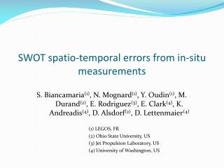
1. S. Biancamaria(1), N. Mognard(1), Y. Oudin(1), M. Durand(2), E. Rodriguez(3), E. Clark(4), K. Andreadis(4), D. Alsdorf(2), D. Lettenmaier(4)‏ (1) LEGOS, FR (2) Ohio State University, US (3) Jet Propulsion Laboratory, US (4) University of Washington, US SWOT spatio-temporal errors from in-situ measurements

2. This study aims to address 2 questions: • What is the error due to the SWOT temporal sampling ? • How accurate can we expect discharge derived from SWOT measurements to be ? • Preliminary estimates of these errors are based on in-situ measurements at stream gauges. • Extend these errors from gauges to the whole rivers (for global estimates).

3. 1. Temporal sampling

4. Purpose of the temporal sampling study • Estimate the maximum errors due to the orbit temporal sampling. • Hypothesis: SWOT measurements have already been converted to discharge. • Focus only on errors for monthly discharge estimates.

5. Methodology (1/2) • Step 1: Estimate the « true » discharge = daily discharge from in-situ gauges (Qt). • Step 2: From daily discharge, extract the discharge at SWOT observation time. 5-day and 10-day discharge have also been extracted. • Step 3: Compute the monthly mean from daily discharge (our « true » monthly mean, Qmt) and from the subsampled discharge (Qmsub).

6. Methodology (2/2) • Step 4:  Compute the error (σt/Q): • Step 5: Compute this error for gauges around the world and classify them as a function of the river drainage area. • Step 6: Fit a relationship between the maximum error and the drainage area.

7. Gauges data used • 201 gauges used from USGS, GRDC, ANA and HyBAM:

8. SWOT orbit data used • Orbit 1: 20 day repeat period, 74° inclination and ~1000km altitude (3 day sub-cycle), • Orbit 2: 22 day repeat period, 78° inclination and ~1000km altitude. • Twodifferentorbits have been considered : Histogram of the SWOT observations for the 201 gaugesr

9. Error vs drainage area for the 201 gauges Maximum error fit (power law)‏

10. Error vs drainage area for the 201 gauges • Very similar errors between the 2 orbits. • Comparison with a constant sub-sampling: • 5 day subsampling = 4 observations in 20 days. • 10 day subsampling = 2 observations in 20 days. • SWOT errors closer to 10day subsampling errors. • Yet SWOT observation number in 20 days: from 2 (at the equator) to 7 and more (at high latitudes).

11. SWOT temporal sampling • Why SWOT errors not closer to 5 day subsampling errors ? • Because SWOT does not have a constant time sampling: SWOT sampling - Equatorial gauges SWOT sampling - Arctic gauges Time period not sampled Very close observations

12. Results summary • Using more than 200 gauges and 2 different SWOT orbits • A fit of the relationship between maximum errors and the drainage area has been computed. • Importance of the SWOT temporal sampling on the monthly discharge.

13. 2. Measurement error

14. Purpose of this study • Rough estimate of the discharge error (using in-situ discharge) due to measurement error. • How the study could be extended to all the rivers. • Methodology (1/2) • Hypothesis: Power law relationship between discharge (Q) and river depth (D): Q=c.Db. • For river depth D=h-h0, h is the elevation measured by SWOT and h0 is the river bed elevation.

15. Methodology (2/2) • The error on the discharge estimates (σQ/Q) is: where σD is SWOT measurement error (σD=10cm)and η is the model error (between in-situ discharge and the discharge from rating curve).

16. Gauges data used • Gauges from USGS, ANA,HyBAM and IWM: 64 gauges in America 10 gauges in Bangladesh

17. Model error (η) vs SWOT measurement error (b.σD/D):

18. Model error (η) vs SWOT measurement error • The SWOT measurement error is low. • Estimate the model error (η) is difficult: most of the discharges come from rating curve (very low error with good fit or high error because of bad fit). • Hypothesis: the model error ~20% (Dingman and Sharma, 1997; Bjerklie et al., 2003).

19. Sensitivity to the b coefficient • Power coefficient b in the power law rating curve depends on bathymetry, difficult to interpolate between gauges. • How is the discharge error sensitive to the b parameter ? with Q=c.Db

20. Sensitivity to the b coefficient • σQ/Q vs D and b (for η =0.2 and σD=10cm): 30% 1.5m with Q=c.Db

21. River Median(b)‏ Amazon 2.0 Bangladeshi 3.2 Colorado 2.5 Mississippi 1.6 Missouri 3.8 All rivers 2.3 Sensitivity to the b coefficient • Median value and histogram of b for the 5 rivers: Coherent with previous studies: Fenton (2001) and Fenton and Keller (2001) found b=2; Chester (1986) found b=2.5.

22. Sensitivity to the b coefficient • σQ/Q computed for each gauge (η =0.2 and σD=10cm): Very low value of D (<80cm)‏

23. Results summary • Using more then 70 gauges with both discharge and water elevation. • The model error (η ) can be assumed ~20%. • Low influence of b on SWOT error for rivers with a depth above 1.5m (for a b coefficient below 3). • b=2 can be used to estimate SWOT measurement globally as it is close to the value found in this study and previous ones.

24. Conclusions • Importance of the SWOT temporal sampling on the computation of monthly discharge. • SWOT spatio-temporal errors have been computed from the in situ networks for different satellite orbits. • General hydrological parameters have been derived from these analysis. • These parameters will be used to generate discharge error maps for a global river network, (see the following talk from Kostas Andreadis).

25. Thankyou for your attention!

26. Results • Tropical rivers (8°N<gauges latitude<20°N )‏ • Equatorial rivers (-13°N<gauges latitude<3°N )‏ • Mid-latitude rivers (33°N<gauges latitude<53°N )‏ • Arcticrivers (50°N<gauges latitude<72°N )‏