Download
1 / 69
710 likes | 938 Views
Properties of the Mobile Radio Propagation Channel. Jean-Paul M.G. Linnartz Department Head CoSiNe Nat.Lab., Philips Research. Statistical Description of Multipath Fading. The basic Rayleigh / Ricean model gives the PDF of envelope But: how fast does the signal fade?

E N D
Properties of the Mobile Radio Propagation Channel Jean-Paul M.G. Linnartz Department Head CoSiNe Nat.Lab., Philips Research
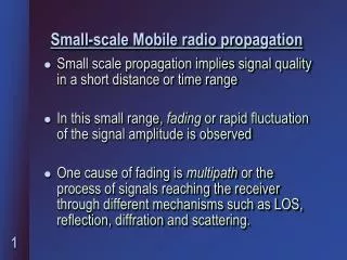
Statistical Description of Multipath Fading The basic Rayleigh / Ricean model gives the PDF of envelope • But: how fast does the signal fade? • How wide in bandwidth are fades? Typical system engineering questions: • What is an appropriate packet duration, to avoid fades? • How much ISI will occur? • For frequency diversity, how far should one separate carriers? • How far should one separate antennas for diversity? • What is good a interleaving depth? • What bit rates work well? • Why can't I connect an ordinary modem to a cellular phone? The models discussed in the following sheets will provide insight in these issues
The Mobile Radio Propagation Channel A wireless channel exhibits severe fluctuations for small displacements of the antenna or small carrier frequency offsets. Amplitude Frequency Time Channel Amplitude in dB versus location (= time*velocity) and frequency
Time Domain Channel variations Delay spread Interpretation Fast Fading InterSymbol Interference Correlation Distance Channel equalization Frequency Doppler spectrum Frequency selective fading Domain Intercarrier Interf. Coherence bandwidth Interpretation Time Dispersion vs Frequency Dispersion Time Dispersion Frequency Dispersion
Two distinct mechanisms 1.) Time dispersion • Time variations of the channel are caused by motion of the antenna • Channel changes every half a wavelength • Moving antenna gives Doppler spread • Fast fading requires short packet durations, thus high bit rates • Time dispersion poses requirements on synchronization and rate of convergence of channel estimation • Interleaving may help to avoid burst errors 2.) Frequency dispersion • Delayed reflections cause intersymbol interference • Channel Equalization may be needed. • Frequency selective fading • Multipath delay spreads require long symbol times • Frequency diversity or spread spectrum may help
Time dispersion of narrowband signal (single frequency) • Transmit: cos(2p fc t) • Receive: I(t) cos(2p fc t) + Q(t) sin(2p fc t) • = R(t) cos(2p fc t + f) • I-Q phase trajectory • As a function of time, I(t) and Q(t) follow a random trajectory through the complex plane • Intuitive conclusion: • Deep amplitude fades coincide with large phase rotations Animate
Doppler shiftand Doppler spread • All reflected waves arrive from a different angle • All waves have a different Doppler shift The Doppler shift of a particular wave is Maximum Doppler shift: fD = fc v / c • Joint Signal Model • Infinite number of waves • First find distribution of angle of arrival, • then compute distribution of Doppler shifts • Uniform distribution of angle of arrival f: fF(f) = 1/2p • Line spectrum goes into continuous spectrum Calculate
Doppler Spectrum If one transmits a sinusoid, … what are the frequency components in the received signal? • Power density spectrum versus received frequency • Probability density of Doppler shift versus received frequency • The Doppler spectrum has a characteristic U-shape. • Note the similarity with sampling a randomly-phased sinusoid • No components fall outside interval [fc- fD, fc+ fD] • Components of + fD or -fD appear relatively often • Fades are not entirely “memory-less”
How do systems handle Doppler Spreads? • Analog • Carrier frequency is low enough to avoid problems (random FM) • GSM • Channel bit rate well above Doppler spread • TDMA during each bit / burst transmission the channel is fairly constant. • Receiver training/updating during each transmission burst • Feedback frequency correction • DECT • Intended to pedestrian use: only small Doppler spreads are to be anticipated for. • IS95 • Downlink: Pilot signal for synchronization and channel estimation • Uplink: Continuous tracking of each signal
Autocorrelation of the signal We now know the Doppler spectrum, but ... how fast does the channel change? • Wiener-Kinchine Theorem: • Power density spectrum of a random signal is the Fourier Transform of its autocorrelation • Inverse Fourier Transform of Doppler spectrum gives autocorrelation of I(t), or of Q(t)
R2 = I2 + Q2 Note: get more elegant expressions for complex amplitude H NB: PDF of the real amplitude R For the amplitude r1 and r2 Correlation:
Autocorrelation of amplitude R2 = I2 + Q2 The solution is known as the hypergeometric function F(a,b;c;z) or, in good approximation, ..
Amplitude r(t0) and Derivative r’(t0) are uncorrelated J0() Correlation is 0 for t = 0
Simulation of multipath channels ? Jakes' Simulator for narrowband channel generate the two bandpass “noise” components by adding many sinusoidal signals. Their frequencies are non-uniformly distributed to approximate the typical U-shaped Dopplerspectrum. N Frequency components are taken at 2p i fi = fm cos -------- 2(2N+1) with i = 1, 2, .., N All amplitudes are taken equal to unity. One component at the maximum Doppler shift is also added, but at amplitude of 1/sqrt(2), i.e., at about 0.707 . Jakes suggests to use 8 sinusoidal signals. Approximation (orange) of the U-Doppler spectrum (Black)
Frequency Dispersion • Frequency dispersion is caused by the delay spread of the channel • Frequency dispersion has no relation to the velocity of the antenna
Typical values of delay spread Picocells 1 .. 2 GHz: TRMS < 50 nsec - 300 nsec • Home 50 nsec • Shopping mall 100 - 200 nsec • Railway station 200 - 450 nsec • Office block 100 - 400 nsec
Typical Delay Profiles For a bandlimited signal, one may sample the delay profile. This give a tapped delay line model for the channel, with constant delay times
COST 207 Typical Urban Reception (TU6) COST 207 describes typical channel characteristics for over transmit bandwidths of 10 to 20 MHz around 900MHz. TU-6 models the terrestrial propagation in an urban area. It uses 6 resolvable paths COST 207 profiles were adapted to mobile DVB-T reception in the E.U. Motivate project. Tap number Delay (us) Power (dB) Fading model 1 0.0 -3 Rayleigh 2 0.2 0 Rayleigh 3 0.5 -2 Rayleigh 4 1.6 -6 Rayleigh 5 2.3 -8 Rayleigh 6 5.0 -10 Rayleigh
COST 207 A sample fixed channel Tap number Delay ( (ms) Amplitude r Level (dB) Phase ( (rad) 1 0.050 0.36 -8.88 -2.875 2 0.479 1 0 0 3 0.621 0.787 -2.09 2.182 4 1.907 0.587 -4.63 -0.460 5 2.764 0.482 -6.34 -2.616 6 3.193 0.451 -6.92 2.863 • COST 207 Digital land mobile radio Communications, final report, September 1988. • European Project AC 318 Motivate: Deliverable 06: Reference Receiver Conditions for Mobile Reception, January 2000
Multipath Channel • Transmit signal s(t) • Received signal r(t) = an gn (t) + n(t), Channel model: Iwreflected waves have the following properties: • Di is the amplitude • Ti is the delay TO DO make math consistent • Signal parameters: • an is the data • c is the carrier frequency
Doppler Multipath Channel Correlation between p-th and q-th derivative TO DO make math consistent
Doppler Multipath Channel TO DO make math consistent
Random Complex-Gaussian Amplitude Special case • This defines the covariance matrix of subcarrier amplitudes at different frequencies • This is used in OFDM for cahnnel estimation TO DO make math consistent
Scatter Function of a Multipath Mobile Channel Gives power as function of · Doppler Shift (derived from angle of arrival f) Excess Delay · Example of a scatter plot Horizontal axes: · x-axis: Excess delay time · y-axis: Doppler shift Vertical axis · z-axis: received power
Freq. and time selective channels • Special cases • Zero displacement / motion: = 0 • Zero frequency separation: f = 0
Wideband Narrowband OFDM Time Time Time Frequency Frequency Frequency Effects of Multipath (I)
DS-CDMA Frequency Hopping MC-CDMA + - + + - + - Time Time Time + - - - + - + - + - - + - + - + Frequency Frequency Frequency Effects of Multipath (II)
BER • BER for Ricean fading calculate
Time Dispersion Revisited The duration of fades
Level crossings per second • Number of level crossing per sec is proportional to • speed r' of crossing R (derivative r' = dr/dt) • probability of r being in [R, R + dR]. This Prob = fR(r) dr
Derivation of Level Crossings per Second • Random process r’ is derivative of the envelope r w.r.t. time • Note: here we need the joint PDF; • not the conditional PDF f(r’½r=R) • We derive f(r’½r=R) from f(r’,r) and f(i1,i2,q1,q2)