Download

1 / 23
240 likes | 412 Views
Approximate Nearest Neighbors and the Fast Johnson-Lindenstrauss Transform. Nir Ailon , Bernard Chazelle (Princeton University). Dimension Reduction. Algorithmic metric embedding technique (R d , L q ) ! (R k , L p ) k << d Useful in algorithms requiring exponential (in d) time/space

E N D
Approximate Nearest Neighborsand theFast Johnson-LindenstraussTransform Nir Ailon, Bernard Chazelle (Princeton University)
Dimension Reduction • Algorithmic metric embedding technique (Rd, Lq) ! (Rk, Lp) k << d • Useful in algorithms requiring exponential (in d) time/space • Johnson-Lindenstrauss for L2 • What is exact complexity?
Dimension Reduction Applications • Approximate nearest neighbor [KOR00, IM98]… • Text analysis [PRTV98] • Clustering [BOR99, S00] • Streaming [I00] • Linear algebra [DKM05, DKM06] • Matrix multiplication • SVD computation • L2 regression • VLSI layout Design [V98] • Learning [AV99, D99, V98] . . .
Three Quick Slides on:Approximate Nearest Neighbor Searching . . .
Approximate Nearest Neighbor P = Set of n points x pmin p dist(x,p) · (1+)dist(x,pmin)
Approximate Nearest Neighbor • d can be very large • -approx beats “curse of dimensionality” • [IM98, H01] (Euclidean), [KOR00] (Cube): • Time O(-2d log n) • Space nO(-2) Bottleneck: Dimension reduction Using FJLT O(d log d + -3 log2 n)
The d-Hypercube Case • [KOR00] • Binary search on distance 2 [d] • For distance multiply space by random matrix2 Z2k £ d k=O(-2 log n)ij i.i.d. » biased coin • Preprocess lookup tables for x (mod 2) • Our observation: can be made sparse • Using “handle” to p2 P s.t. dist(x,p) • Time for each step: O(-2d log n) ) O(d + -2 log n) How to make similar improvement for L2 ?
History of Johnson-LindenstraussDimension Reduction [JL84] • : Projection of Rd onto random subspace of dimension k=c-2 log n • w.h.p.:8 pi,pj2 P || pi - pj ||2 = (1±O()) ||pi - pj||2 • L2! L2 embedding
History of Johnson-LindenstraussDimension Reduction [FM87], [DG99] • Simplified proof, improved constant c • 2 Rk £ d : random orthogonal matrix 1 ||i||2=1 i¢j = 0 2 k
History of Johnson-LindenstraussDimension Reduction [IM98] • 2 Rk£ d : ij i.i.d. » N(0,1/d) 1 E ||i||22=1 E i¢j = 0 2 k
History of Johnson-LindenstraussDimension Reduction [A03] • Need only tight concentration of |i¢ v|2 • 2 Rk£ d : ij i.i.d. » +1 1/2 -1 1/2 1 E ||i||22=1 E i¢j = 0 2 k
History of Johnson-LindenstraussDimension Reduction [A03] • 2 Rk£ d : ij i.i.d. » • Sparse +1 1/6 0 2/3 -1 1/6 1 E ||i||22=1 E i¢j = 0 2 k
Sparse Johnson-Lindenstrauss • Sparsity parameter: s = Pr[ ij 0 ] • Cannot be o(1) due to “hidden coordinate” 0 0 0 0 0 0 0 0 0 0 0 0 0 0 0 0 0 0 0 0 0 0 0 0 1 0 0 v = 2 Rd 0 0 0 0 0 0 0 0 0 0 0 0 0 0 0 0 0 0 0 0 0 0 0 0 0 0 0 0 0 0 0 0 0 0 0 0 0 0 0 0 0 0 0 0
Uncertainty Principle ^ v sparse ) v dense v = H v ^ • - Walsh - Hadamard matrix • - Fourier transform on {0,1}log2 d • Computable in time O(d log d) • Isometry: ||v||2 = ||v||2 ^
Adding Randomization • H deterministic, invertible) We’re back to square one! • Precondition H with random diagonal D ±1 ±1 ±1 D = . . . • - Computable in time O(d) • Isometry
The l1-Bound Lemma • w.h.p.:8 pi,pj2 P µ Rd : ||HD(pi - pj)||1· O(d-1/2 log1/2 n) ||pi - pj||2 • Rules out: HD(pi – pj) = “hidden coordinate vector” !! instead...
Hidden Coordinate-Set Worst-case v = pi - pj (assuming l1-bound): • 8 j J: |vj| = (d-1/2 log1/2 n) 8 jJ: vj= 0 J µ [d], |J| = (d/log n) (assume ||v||2 = 1)
Fast J-L Transform FJLT = H D ij i.i.d» Sparse JL Diag(±1) Hadamard 0 1-s N(0,1) s l2! l2 l2! l1 -1 log n log2 n s s d d Bottleneck: Bias of |i¢ v| Bottleneck: Variance of |i¢ v|2
Applications • Approximate nearest neighbor in (Rd, l2) • l2 regression: minimize ||Ax-b||2A 2 Rn £ d over-constrained: d<<n [DMM06] approximate by sampling [Sarlos06] using FJLT ) constructive • More applications...? non-constructive
Interesting Problem I Improvement & lower bound for J-L computation
Interesting Problem II • Dimension reduction is sampling • Sampling by random walk: • Expander graphs for uniform sampling • Convex bodies for volume estimation • [Kac59]: Random walk on orthogonal groupfor t=1..T: pick i,j 2R [d], 2R [0,2) vi vi cos + vj sin vj -vi sin+ vj cos • Output (v1, ..., vk) as dimension reduction of v • How many steps for J-L guarantee? • [CCL01], [DS00], [P99] . . . Thank You ! Ã