Download
1 / 29
300 likes | 599 Views
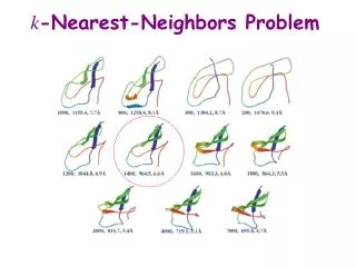
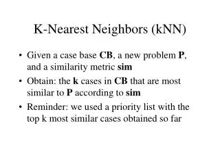
K-Nearest Neighbors (kNN). Given a case base CB , a new problem P , and a similarity metric sim Obtain: the k cases in CB that are most similar to P according to sim Reminder: we used a priority list with the top k most similar cases obtained so far. Forms of Retrieval.

E N D
K-Nearest Neighbors (kNN) • Given a case base CB, a new problem P, and a similarity metric sim • Obtain: the k cases in CB that are most similar to P according to sim • Reminder: we used a priority list with the top k most similar cases obtained so far
Forms of Retrieval • Sequential Retrieval • Two-Step Retrieval • Retrieval with Indexed Cases
Retrieval with Indexed Cases Sources: Bergman’s b`ook Davenport & Prusack’s book on Advanced Data Structures Samet’s book on Data Structures
Red light on? Yes Beeping? Yes … Transistor burned! Range Search Space of known problems
K-D Trees • Idea: Partition of the case base in smaller fragments • Representation of a k-dimension space in a binary tree • Similar to a decision tree: comparison with nodes • During retrieval: • Search for a leaf, but • Unlike decision trees backtracking may occur
Definition: K-D Trees • Given: • K types: T1, …, Tk for the attributes A1, …, Ak • A case base CB containing cases in T1 … Tk • A parameter b (size of bucket) • A K-D tree T(CB) for a case base CB is a binary tree defined as follows: • If |CB| < b then T(CB) is a leaf node (a bucket) • Else T(CB) defines a tree such that: • The root is marked with an attribute Ai and a value v in Ai and • The 2 k-d trees T({c CB: c.i-attribute < v}) and T({c CB: c.i-attribute v}) are the left and right subtrees of the root
P(32,45) Example A1 (0,100) <35 35 (60,75) Toronto Denver Omaha A2 (80,65) Buffalo <40 (5,45) Denver (35,40) Chicago 40 Atlanta (85,15) A1 (50,10) Mobile <85 (25,35) Omaha 85 (90,5) Miami Atlanta Miami Mobile (0,0) (100,0) A1 • Notes: • Supports Euclidean distance • May require backtracking • Closest city to P(32,45)? • Priority lists are used for computing kNN <60 60 Toronto Buffalo Chicago
Variant: InReCA Tree Ai unknown v1 vn … v2 Ai unknown v1 … >vn >v1 v2 Can be combined with numeric attributes Using Decision Trees as Index Standard Decision Tree Ai vn … v1 v2 • Notes: • Supports Hamming distance • May require backtracking • Operates in a similar fashion as kd-trees • Priority lists are used for computing kNN
Variation: Point QuadTree • Particularly suited for performing range search (i.e, similarity assessment) • Adequate with fewer numerical and known-important attributes • A node in a (point) quadtree contains: • 4 Pointers: quad [‘NW’], quad [‘NE’], • quad[‘SW’], and quad[‘SE’] • point, of type DataPoint, which in turn contains: • name • (x,y) coordinates
Example (0,100) (60,75) Toronto (80,65) Buffalo (5,45) Denver (35,40) Chicago Atlanta (85,15) (50,10) Mobile (25,35) Omaha (90,5) Miami (0,0) (100,0) Insertion order: Chicago, Mobile, Toronto, Buffalo, Denver, Omaha, Atlanta and Miami
Insertion in Quadtree Chicago Denver Omaha Mobile Toronto Atlanta Miami Buffalo
Insertion Procedure We define a new type: quadrant: ‘NW’, ‘NE’, ‘SW’, ‘SE’ function PT_compare(DataPoint dP, dR): quadrant //quadrant where dP belongs relative to dR if (dP.x < dR.x) then if (dP.y < dR.y) thenreturn ‘SW’ elsereturn ‘NW’ else if (dP.y < dR.y) then return ‘SE’ else return ‘NE’
Insertion Procedure (Cont.) procedure PT_insert(Pointer P, R) //inserts P in the tree rooted at R Pointer T //points to the current node being examined Pointer F // points to the parent of T Quadrant Q //auxiliary variable T R F null while not(T == null) && not(equalCoord(P.point,T.point)) do F T Q PT_compare(P.point, T.point) T T.quad[Q] if (T == null) then F.quad[Q] P
Search Typical query: “find all cities within 50 miles of Washington,DC” In the initial example: “find all cities within 8 data units from (83,13)” • Solution: • Discard NW, SW and NE of Chicago (that is, only examine SE) • There is no need to search the NW and SW of Mobile
Search (II) Let R be the root of the quadtree, what regions need to be inspected if R is in the quadrant: 1 2 3 9 10 r 5 4 A 1: SE 11 12 2: SW, SE 6 8 7 8: NW 11: NW, NE, SE
Priority Queues • Typical example: printing in a Unix/Linux environment. Printing jobs have different priorities. • These priorities may override the FIFO policy of the queues (i.e., jobs with the highest priorities will get printed first). • Operations supported in a priority queue: • Insert a new element • Extract/Delete of the element with the lowest priority • In search trees, the priority is based on the distance • Insertion, deletion can be done in O(Log N) and look-head in O(1)
Nearest-Neighbor Search Problem: Given a point quadtree T and a point P find the node in T that is the closest to P Idea: traverse the quadtree maintaining a priority list, candidates, based on the distance from P to the quadrants containing the candidate nodes (60,75) Toronto (80,65) Buffalo (5,45) Denver (35,40) Chicago (85,15) Atlanta P(95,15) (50,10) Mobile (25,35) Omaha (90,5) Miami
Distance from P to a Quadrant Let f-1 be the inverse of the distance-similarity compatible function P2 P3 2 distance(P,SW) = f-1(sim(P,(P.y,0)) 3 (x,y) distance(P,NW) = f-1(sim(P,(x,y)) 4 P1 P 1 P4 distance(P,NE) = f-1(sim(P,(P.x,0)) distance(P,SE) = 0
Idea of the Algorithm Candidates = [Chicago (4225)] Buffer: null () (60,75) Toronto (5,45) Denver (35,40) Chicago P = (95,15) (50,10) Mobile (25,35) Omaha Candidates = [Mobile(0),Toronto (25), Omaha (60), Denver(4225)] Buffer: Chicago (4225)
List of Candidates • Termination test: Buffer.distance < distance(candidates.top,P) • if “yes” then return Buffer • if “no” then continue • In this particular example, is “no” since Mobile is closer to P than Chicago • Examine the quadrant of the top of candidates (Mobile) and make it the new buffer: distance(P,NE) = 0 distance(P,SE) = 5 (85,15) Atlanta P(95,15) (50,10) Mobile (90,5) Miami Buffer: Mobile (1625)
Finally the Nearest Neighbor is Found Candidates = [Atlanta(0), Miami(5), Toronto (25), Omaha (60), Denver(4225)] Buffer: Atlanta(100) A new iteration: Candidates = [Miami(5), Toronto (25), Omaha (60), Denver(4225)] The algorithm terminates since the distance from Atlanta to P is less than the distance from Miami to P
Complexity • Experiments show that random insertion of N nodes is roughly O(N log4N) • Thus, insertion of a single node is O(log4N) • But worst case (actual complexity) can be much worse • Range search can be performed in O(2 N ½)
Delete • First idea: • Find the node N that you want to delete • Delete N and all of its descendants ND • For each node N’ in ND, add N’ back into the tree Terrible idea; it is too inefficient!.
Idealized Deletion in Quadtrees If a point A is to be deleted find a point B such that the region between A and B is empty and replaced A with B B “Hatched Region” A Why? Because all the remaining points will be in the same quadrants relative to B as they are relative to A. For example, Omaha could replace Chicago as the root.
F C A E D Problem with Idealized Situation First Problem: A lot of effort is required to find such a B. In the following example which point (C, F, D or A) has a hatched region with A? Answer: none!. Second problem: No such a B may exit!
NW NE SW NW SW NE SE NE SW SE Problem with Defining a New Root Several points will have to be re-positioned Old root New root
Deletion Process Delete P: 1. If P is a leaf then just delete it!. 2. If P has a single child C, then replace P with C 3. For all other cases: 3.1 Compute 4 candidate nodes, one for each quadrant under P 3.2 Select one of the candidate node, N according to certain criteria 3.3 Delete several nodes under P and collect them in a list, ADD. Also delete N. 3.4 Make N.point the new root: P.point N.point 3.5 Re-insert all nodes in ADD
A Word of Warning About Deletion • In databases frequently deletion is not done immediately because it is so time-consuming. • Sometimes they don’t even do insertions immediately! • Instead they keep a log with all deletions (and additions), and periodically (i.e., every night, weekend), the log is traversed to update the database. The technique is called Differential Databases. • Deleting cases is part of the general problem of case base maintenance.
Properties of Retrieval with Indexed Cases • Advantage: • Disadvantages: • Efficient retrieval • Incremental: don’t need to rebuild index again every time a new case is entered • -error does not occur • Cost of construction is high • Only work for monotonic similarity relations