Download
1 / 29
330 likes | 641 Views
Chapter 13. Aggregate Demand in the Open Economy We will not cover the Appendix. Homework : pp. 388-89 # 1, 2 or 3 macromodel mundell_fleming # 1, 4, 10 Link to syllabus. Preview of Coming Attractions! Fig. 13-3, p. 361. The Mundell -Fleming Model.

E N D
Chapter 13. Aggregate Demand in the Open EconomyWe will not cover the Appendix. Homework: pp. 388-89 # 1, 2 or 3 macromodelmundell_fleming # 1, 4, 10 Link to syllabus
Preview of Coming Attractions!Fig. 13-3, p. 361. The Mundell-Fleming Model
Mundell and Dornbusch RudigerDornbusch 1942-2002. Robert Mundell, 1932- Nobel prize 1999 Mundell taught at U. of Chicago for many years, where Dornbusch was his student. Dornbusch taught at MIT.
Fig. 13-2, p. 360. The LM* Curve With a vertical LM*, all the fun is over before we even start.
Fig. 13-3 p. 361. Equilibrium in the Mundell Fleming Model Appreciation of US $ Depreciation of US $
Fond, old memories. When the textbook expanded from the closed economy loanable funds model of Chapter 3 to the open economy loanable funds model of Chapter 6, it kept the same general framework, but we ended up with two graphs; one with r on the vertical axis [where r always equaled r*], and the other with the exchange rate on the vertical axis. Now, from chapter 12 to13, we go from closed economy IS-LM to open economy IS-LM. This time, however, we don’t bother with the graph that has r on the vertical axis, but jump right into the graph with the exchange rate on the vertical axis.
Fig. 13-4, p. 362. Fiscal Expansion Under Floating Exchange Rates No change in output without even assuming a vertical AS curve.
mt’s attempt at explaining result of fiscal expansion(assuming small open economy, flexible x-rates) An increase in government expenditures → would raise interest rates, → leading to an inflow of foreign capital (loans), → appreciating the currency (higher Y/$), → lowering net exports, → which cancels out the expansionary effect of higher Gov’t spending → leaving the economy at the same level of output. Another part of the story is that these effects are so strong that the domestic interest rate never really rises above the world interest rate.
Fig. 13-5, p. 364. Monetary Expansion under Floating Exchange Rates
mt‘s attempt at explaining this result of monetary expansion The increase in the money supply would initially → lower domestic interest rates, and so → cause capital outflows and depreciate the currency → raise net exports, increasing real output
Fig. 13-6, p. 365. Trade Restriction under Floating Exchange Rates
Fig. 13-7, p. 367. How a Fixed Exchange Rate Governs the Money Supply
Fig. 13-7, p. 367 (again). How a Fixed Exchange Rate Governs the Money Supply A 180 150 120 150 H At point A, agents borrow$ and convert them to yen at 180Y/$ overseas, then bring the Yen for exchange in the US, buying $ at 150 for an automatic profit. The Fed, in selling $, raises US money supply. At H, agents will buy $ at 120 and sell them to the Fed at 150Y/$, making 25 % profit. This reduces the supply of $, pushing the LM* to the left.
Fig. 13-8, p. 369. Fiscal Expansion under Fixed Exchange Rates
Fig. 13-9, p. 369. Monetary Expansion under Fixed Exchange Rates Monetary policy has no effect with fixed exchange rates, for a s.o.e.
Fig. 13-10, p. 371. Trade Restriction under Fixed Exchange Rates
Appendix The large open economy is an average of the closed economy and the small open economy. To find how any policy will affect any variable, find the answer in the extreme cases for the closed and SOE, and take the ‘average’. (page 394)
Figure 13.15 p. 391 (appendix). A Short-Run Model of a Large Open Economy
Figure 13.16 p. 392. A Fiscal Expansion in a Large Open Economy An increase in Gov’t spending raises real GDP and the real interest rate, lowers capital outflows, raises the exchange rate, and reduces net exports. The decline in net exports lowers the increase of real GDP. In the SOE, there is no change in GDP because the ∆ G = - ∆ NX.
Figure 13.17 p. 393. A Monetary Expansion in a Large Open Economy An increase in M moves LM right, lowering r. This increase capital outflow, which lowers the exchange rate, ultimately increasing net exports. In a SOE, an increase in M increases real output in the short run.