Download
1 / 36
360 likes | 475 Views
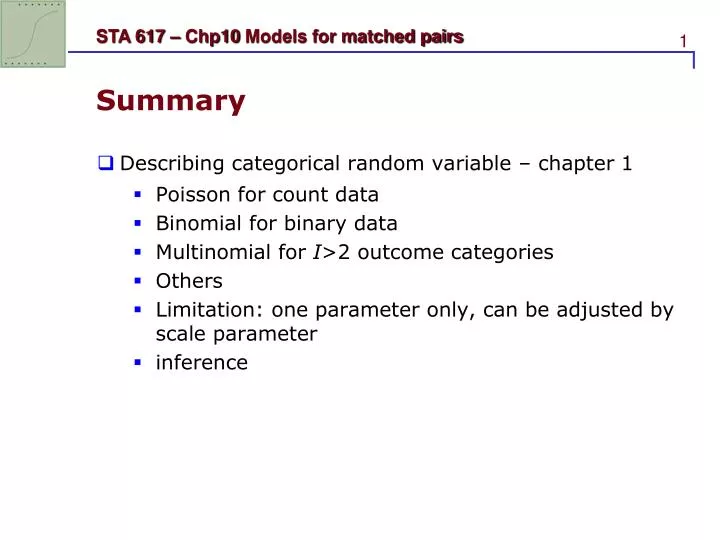
Summary. Describing categorical random variable – chapter 1 Poisson for count data Binomial for binary data Multinomial for I >2 outcome categories Others Limitation: one parameter only, can be adjusted by scale parameter inference. Summary. Two-way contingency table – chapters 2, 3

E N D
Summary • Describing categorical random variable – chapter 1 • Poisson for count data • Binomial for binary data • Multinomial for I>2 outcome categories • Others • Limitation: one parameter only, can be adjusted by scale parameter • inference
Summary • Two-way contingency table – chapters 2, 3 • Parameters: risk, odds • Comparison: relative risk, odds ratio • Estimation: delta method • Tests: chi-square, fisher’s exact test • Ordered two-way tables: • assign scores - Trend test M2=(n-1)r2 • uses an ordinal measure of monotone trend: • SAS: proc freq with option relarisk, chisq, exact, etc.
Summary • Three-way (multi-way) tables – chapter 2, 3 • Partial tables • Conditional and marginal odds ratio • Conditional and marginal independence • Inference – chapter 4-9: • Third or others variables are considered as covariates • modeling
Summary – generalized linear models • Random component is exponential family (not necessary normal) • Systematic component – linear model • Link function – connect mean to Systematic component xbeta • Log • Logit • Identity
Logistic regression • Chapters 5-7 • SAS proc logistic, genmod • Binary outcome – logistic regression • Multinomial response • Nominal-baseline-category logit models • Ordinal – cumulative logit models
Log-linear model • Chapters 8-9 • Two-way table • Three-way tables • Multi-way tables • Model selection • Ordinal responses • Log-linear model for rates • SAS: genmod
By far – cross sectional data • If the data are collected over time, the data for the same subject in different time points will be correlated. • Longitudinal data • Multivariate responses * • Non-linear models *
Longitudinal data • Chapter 10 – two time points: matched pairs • Chapter 11 – repeated measures using marginal models (no random effects) • Chapter 12 – random effect model or generalized linear mixed models • Recent developments – publications for categorical responses since 2002 (final project) • Read one or two recent papers • 20 minutes presentation
models • Linear model (LMs) (t-tests, ANOVA, ANCOVA) • SAS: proc TTEST, ANOVA, REG, GLM • Generalized linear models (GLMs) • SAS: proc GENMOD, LOGISTIC, CATMOD • Linear mixed model (LMMs) – permitting heterogeneity of variance, variance structure is based on random effects and their variance components • SAS: proc MIXED • Generalized linear mixed models (GLMMs) • SAS: proc NLMIXED • Non-linear mixed model • SAS: proc NLMIXED
Models for matched pairs • In this chapter, we introduce methods for comparing categorical responses for two samples when each observation in one sample pairs with an observation in the other. • For easy understanding, we assume n independent subjects and let Yi = (Yi1,Yi2, ...,Yiti)is the observation of subject i at different time. • In statistics, {Y1,Y2, ...,Yn} are called longitudinal data • For fixed i , Yiis a time series; for fixed time j , {Y1j ,Y2j , ...,Ynj} isa sequence of independent random variables. • If ti = 2 for all i , {Y1,Y2, ...,Yn} is called matched-pairs data. Note that the two samples {Y11,Y21, ...,Yn1} and {Y12,Y22, ...,Yn2} are not independent.
Outline 10.1 Comparing Dependent Proportions; 10.2 Conditional Logistic Regression for Binary Matched Pairs; 10.3 Marginal Models for Squared Contingency Tables; 10.4 Symmetry, Quasi-symmetry and Quasi-independence; 10.5 Measure Agreement Between Observers; 10.6 Bradley-Terry Models for Paired Preferences.
SAS code /*section 10.1.2 page 411*/ data tmp; p11=794/1600; p12=150/1600; p21=86/1600; p22=570/1600; p1plus=p11+p12; pplus1=p11+p21; se=sqrt( ((p12+p21)-(p12-p21)**2)/1600); lci=p1plus-pplus1-1.96*se; uci=p1plus-pplus1+1.96*se; z0=(86-150)/(86+150)**0.5; McNemarsTest=z0**2; pvalue=1-cdf('chisquare',McNemarsTest,1); se_ind=sqrt(p1plus*(1-p1plus)+p1plus*(1-p1plus))/sqrt(1600); /*assume independent*/ lci_ind=p1plus-pplus1-1.96*se_ind; uci_ind=p1plus-pplus1+1.96*se_ind; procprint; run;
SAS code McNemar’s Test data matched; input first second count @@; datalines; 1 1 794 1 2 150 2 1 86 2 2 570 ; proc freq; weight count; tables first*second/ agree; exact mcnem; /*McNemars Test*/ proc catmod; weight count; response marginals; model first*second= (1 0 , 1 1) ; run;
PROC FREQ • For square tables, the AGREE option in PROC FREQ provides the McNemar chi-squared statistic for binary matched pairs, the X2test of fit of the symmetry model (also called Bowker’s test), and Cohen’s kappa and weighted kappa with SE values. • The MCNEM keyword in the EXACT statement provides a small-sample binomial version of McNemar’s test. • PROC CATMOD provide the confidence interval for the difference of proportions. • The code forms a model for the marginal proportions in the first row and the first column, specifying a model matrix in the model statement that has an intercept parameter (the first column) that applies to both proportions and a slope parameter that applies only to the second; hence the second parameter is the difference between the second and first marginal proportions.
Fit marginal model data matched1; input case occasion response count @@; datalines; 1 0 1 794 1 1 1 794 2 0 1 150 2 1 0 150 3 0 0 86 3 1 1 86 4 0 0 570 4 1 0 570 ; proclogisticdata=matched; weight count; model response=occasion; run; Xt proc genmod data=matched1 DESCENDING; weight count; model response=occasion/dist=bin link=identity;
Matlab code for deriving previous MLE and SE %% page 417 syms bn21n12 LL=log(exp(b)^n21/(1+exp(b))^(n12+n21)); simplify(diff(LL,'b')) %result (n21-exp(b)*n12)/(1+exp(b)) %thus beta=log(n21/n12) simplify(diff(diff(LL,'b'),'b')) %result -exp(b)*(n12+n21)/(1+exp(b))^2
10.2.4 Random effects in binary matched-pairs model • An alternative remedy to handling the huge number of nuisance parameters in logit model (10.8) treats as random effects. • Assume ~ • This model is an example of a generalized linear mixed model, containing both random effects and the fixed effect beta. • Fit by proc NLMIXED • Chapter 12
10.2.5 Logistic Regression for Matched Case–Control Studies • The two observations in a matched pair need not refer to the same subject. • For instance, case-control studies that match a single control with each case yield matched-pairs data. • Example: A case-control study of acute myocardial infarction (MI) among Navajo Indians matched 144 victims of MI according to age and gender with 144 people free of heart disease.
Now, for subject t in matched pair i, consider the model • the conditional ML estimate of OR is
10.2.6 Conditional ML for matched pairs with multiple predictors
10.2.7 Marginal models vs. conditional models • Section 10.1 Marginal model (McNemar’s test H0: =0) • Section 10.2 conditional model • Conditional ML • Random effects, NLMIXED