Download
1 / 46
460 likes | 613 Views
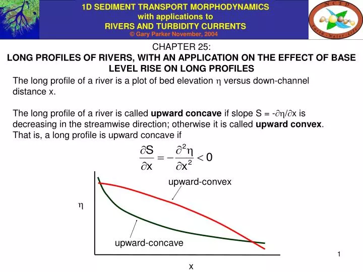
CHAPTER 25: LONG PROFILES OF RIVERS, WITH AN APPLICATION ON THE EFFECT OF BASE LEVEL RISE ON LONG PROFILES. The long profile of a river is a plot of bed elevation versus down-channel distance x.

E N D
CHAPTER 25: LONG PROFILES OF RIVERS, WITH AN APPLICATION ON THE EFFECT OF BASE LEVEL RISE ON LONG PROFILES The long profile of a river is a plot of bed elevation versus down-channel distance x. The long profile of a river is called upward concaveif slope S = -/x is decreasing in the streamwise direction; otherwise it is called upward convex. That is, a long profile is upward concave if
LONG PROFILE OF THE AMAZON RIVER The Amazon River shows a rather typical long profile. Note that it is upward concave almost everywhere. The data are from Pirmez (1994).
TRANSIENT LONG PROFILES In Chapter 14 we saw that in an idealized equilibrium, or graded state rivers have constant slopes in the downstream direction, adjusted so that the rate of inflow of sediment to a reach equals the rate of outflow. When more sediment is fed in than flows out, the river is forced to aggrade toward a new equilibrium. During this transient period of aggradation the profile is upward-concave. A sample calculation showing this (and performed with RTe-bookAgDegNormal.xls) is given below. Likewise, when more sediment flows out of the reach than is fed in, the river is forced to degrade toward a new equilibrium. During this transient period of degradation the profile is upward-convex. (Try a run and see.)
QUASI-EQUILIBRIUM LONG PROFILES • The long profiles of long rivers generally approach an upward-concave shape that is maintained as a quasi-equilibrium form over long geomorphic time. As the word “quasi” implies, this “equilibrium” is not an equilibrium in the sense that sediment output equals input over each reach. • Reasons for the maintenance of this quasi-equilibrium are summarized in Sinha and Parker (1996). Several of these are listed below. • Subsidence • Sea level rise • Delta progradation • Downstream sorting of sediment • Abrasion of sediment • Effect of tributaries
SUBSIDENCE As a river flow into a subsiding basin, the river tends to migrate across the surface, filling the hole created by subsidence. As a result, the sediment output from a reach is less than the input, and the profile is upward-concave over the long term (e.g. Paola et al., 1992). Rivers entering a (subsiding) graben in eastern Taiwan. Image from NASA website: https://zulu.ssc.nasa.gov/mrsid/mrsid.pl
SEA LEVEL RISE Rivers entering the sea have felt the effect of a 120 m rise in sea level over about 12,000 years at the end of the last glaciation. The rise in sea level was caused by melting glaciers. The effect of this sea level rise was to force aggradation, with more sediment coming into a reach than leaving. This has helped force upward-concave long profiles on such rivers. Sea level rise from 19,000 years BP (before present) until 3,000 years BP according to the Bard Curve (see Bard et al., 1990).
DELTA PROGRADATION Even when the body of water in question (lake or the ocean) maintains constant base level, progradation of a delta into standing water forces long-term aggradation and an upward-concave profile. Missouri River prograding into Lake Sakakawea, North Dakota. Image from NASA website: https://zulu.ssc.nasa.gov/mrsid/mrsid.pl
DOWNSTREAM SORTING OF SEDIMENT Rivers typically show a pattern of downstream fining. That is, characteristic grain size gets finer in the downstream direction. This is because in a sediment mixture, finer grains are somewhat easier to move than coarser grains. Since finer grains can be transported by the same flow at lower slopes, the result is a tendency to strengthen the upward concavity of the profile. Long profile and median sediment grain size on the Mississippi River, USA. Adapted from USCOE (1935) and Fisk (1944) by Wright and Parker (in press).
ABRASION OF SEDIMENT In mountain rivers containing gravel of relatively weak lithology, the gravel tends to abrade in the streamwise direction. The product of abrasion is usually silt with some sand. As the gravel gets finer, it can be transported at lower slopes. The result is tendency to strengthen the upward concavity of a river profile. The image shows a) the long profile of the Kinu River, Japan and b) the profile of median grain size in the same river. The gravel easily breaks down due to abrasion. The river undergoes a sudden transition from gravel-bed to sand-bed before reaching the sea. Image adapted from Yatsu (1955) by Parker and Cui (1998).
EFFECT OF TRIBUTARIES As tributaries enter the main stem of a river, they tend to increase the supply of water more than they increase the supply of sediment, so that the concentration of sediment in the main stem tends to decline in the streamwise direction. Since the same flow carries less sediment, the result is a tendency toward an upward-concave profile. Image courtesy John Gray, US Geological Survey.
UPWARD-CONCAVE LONG PROFILE DRIVEN BY RISING SEA LEVEL The Fly-Strickland River System in Papua New Guinea has been profoundly influenced by Holocene sea level rise. Fly River Strickland River Fly River Image from NASA website: https://zulu.ssc.nasa.gov/mrsid/mrsid.pl
Downchannel reach length L is specified; x = L corresponds to the point where sea level is specified. • The river is assumed to have a floodplain width Bf that is constant, and is much larger than bankfull width Bbf. • The river is sand-bed with characteristic size D. • All the bed material sediment is transported at rate Qtbf during a period constituting (constant) fraction If of the year, at which the flow is approximated as at bankfull flow, so that the annual yield = IfQtbf. • Sediment is deposited across the entire width of the floodplain as the channel migrates and avulses. For every mass unit of bed material load deposited, mass units of wash load are deposited in the floodplain. • Sea level rise is constant at rate . For example, during the period 5,000 – 17,000 BP the rate of rise can be approximated as 1 cm per year. • The river is meandering throughout sea level rise, and has constant sinuosity . • The flow can be approximated using the normal-flow assumptions. (But the analysis easily • generalizes to a full backwater formulation.) FORMULATION OF THE PROBLEM: ASSUMPTIONS
BED MATERIAL LOAD AND WASH LOAD Sea level rise forces a river bed to aggrade. This in turn forces the river to spill out more often onto the floodplain, and therefore forces floodplain aggradation as well. Wash load is by definition contained in negligible quantities in the bed of a river, but is invariably a major constituent of floodplain deposits, and is often the dominant one. That is, wash load could be more accurately characterized as “floodplain material load.” In large sand-bed rivers, for example, the floodplain often contains a lower layer in which sand dominates and an upper layer in which silt dominates. A precise mass balance for wash load is beyond the scope of this chapter. For simplicity it is assumed that for every unit of sand deposited in the channel/floodplain system in response to sea level rise, units of wash load are deposited, where is a specified constant that might range from 0 to 3 or higher. It is assumed that the supply of wash load from upstream is always sufficient for deposition at such a rate. This is not likely to be strictly true, but should serve as a useful starting assumption. In addition, it is assumed for simplicity that the porosity of the floodplain deposits is equal to that of the channel deposits. In fact the floodplain deposits are likely to have a lower porosity.
FORMULATION OF THE PROBLEM: EXNER Sediment is carried in channel but deposited across the floodplain due to aggradation forced by sea level rise. Adapting the formulation of Chapter 15, where qtbf denotes the bankfull (flood) value of volume bed material load per unit width qt, qwbf denotes the bankfull (flood) value of volume wash load per unit width and denotes channel sinuosity,
FORMULATION OF THE PROBLEM: EXNER contd. It is assumed that for every one unit of bed material load deposited units of wash load are deposited to construct the channel/floodplain complex; Thus the final form of Exner becomes
FORMULATION OF THE PROBLEM: MORPHODYNAMIC EQUATIONS Relation for sediment transport: Using the formulation of Chapter 24 for sand-bed streams, Expressing the middle relation in dimensioned forms and solving for Qtbf as a function of S and Qbf, Note that according to this relation the bed material transport load Qtbf is a linear function of slope.
REDUCTION OF THE EXNER EQUATION The Exner equation can be expressed as Reducing with the sediment transport relation it is found that where d denotes a kinematic sediment diffusivity. Note that the resulting form is a linear diffusion equation.
DECOMPOSITION OF THE SOLUTION FOR BED ELEVATION The bed elevation at specified point x = L is set equal to sea level elevation, so that where do denotes sea level elevation at time t = 0, Bed elevation (x,t) is represented in terms of this downstream elevation approximated by sea level and the deviation dev(x,t) = - (L,t) it, so that The problem is solved over reach length L where x = 0 denotes the upstream length and x = L is the point where the river meets the sea. From the above relations, then, Substituting the second of the above relations into the Exner formulations of the previous page yields the forms
BOUNDARY CONDITIONS The upstream boundary condition is that of a specified sediment feed rate Qtbf,feed (during floods) at x = 0. That is, The downstream boundary condition, i.e. is somewhat unrealistic in that L is a prescribed constant. In point of fact, rivers flowing into the sea end in deltas. The topset-foreset break of the delta, where x = L, can move seaward as the delta progrades at constant water surface elevation, and can move seaward or landward under conditions of rising or falling sea level. These issues are examined in more detail in a future chapter.
SOLUTION FOR STEADY-STATE AGGRADATION IN RESPONSE TO SEA LEVEL RISE The case illustrated below is that of steady-state aggradation, with every point aggrading at the rate in response to sea level rise at the same constant rate. In such a case dev becomes a function of x alone, and the problem reduces to
SOLUTION FOR STEADY-STATE AGGRADATION IN RESPONSE TO SEA LEVEL RISE contd. The Exner equation thus reduces to the form which integrates with the upstream boundary condition of the previous page to That is, the bed material load decreases linearly down the channel due to steady-state aggradation forced by sea-level rise. The sediment delivery rate to the sea Qtbf,,sea is given as
SOLUTION FOR STEADY-STATE AGGRADATION IN RESPONSE TO SEA LEVEL RISE contd. Further reducing, Between this relation and the load relation it is seen that where Su denotes the upstream slope at x = 0. That is, slope declines downstream, defining an upward concave long profile.
SOLUTION FOR STEADY-STATE AGGRADATION IN RESPONSE TO SEA LEVEL RISE contd. Now S = - d/dx = - ddev/dx . Making dev and x dimensionless with L as follows results in the equation given below for elevation profile. Integrating subject to the boundary condition dev(L) = 0, or thus the following parabolic solution for long profile is obtained;
REVIEW OF THE STEADY-STATE SOLUTION The parameter EH = 0.05 for the Engelund-Hansen relation, and for sand-bed rivers form* can be approximated as 1.86. Reach length L, bed porosity p, floodplain width Bf, channel sinuosity , intermittency If friction coefficient Cf and the ratio of wash load deposited to bed material load deposited must be specified. The steady-state long profile can then be calculated for any specified values of upstream flood bed material feed rate Qtbf,feed and rate of sea level rise .
REVIEW OF THE STEADY-STATE SOLUTION contd. The predicted streamwise variation in channel bankfull width Bbf and depth Hbf are given from the relations or in dimensioned terms In the absence of tributaries, decreasing bed material load in the streamwise direction causes a decrease in bankfull width Bbf and an increase in bankfull depth Hbf.
CHARACTERISTICS OF THE STEADY-STATE SOLUTION The parameter has a specific physical meaning. The mean annual feed rate of bed material load Gt,feed available for deposition in the reach is given as When wash load is included, the mean annual rate Gfeed available for deposition becomes Valley length Lv is given as The tons/s of sediment Gfill required to fill a reach with length Lv and width Bf with sediment at a uniform aggradation rate in m/s is given as It follows that That is if > 1 then the there is not enough sediment feed over the reach to fill the space created by sea level rise, and the sediment transport rate must drop to zero before the shoreline is reached. If < 1 the excess sediment is delivered to the sea.
CHARACTERISTICS OF THE STEADY-STATE SOLUTION contd. As a result of the above arguments, meaningful solutions are realized only for the case 1. In such cases there is excess sediment to deliver to the sea. In actuality, part of this sediment would be used to prograde the delta of the river, so increasing reach length L. Delta progradation is considered in more detail in a subsequent chapter. If for a given rate of sea level rise it is found that > 1 for reasonable values of reach length L, floodplain width Bf and sediment feed rate Gfeed, no steady state solution exists for that rate of sea level rise. The implication is that the entire profile, including the position of the delta, must migrate upstream, or transgress. A model of this transgression is developed in a subsequent chapter.
SAMPLE CALCULATION The calculation is implemented in the spreadsheet workbook RTe-bookSteadyStateAg.xls. The following sample input parameters are used in the succeeding plots. It should be noted that a sea level rise of 10 mm/year forces a rather extreme response.
CAN THE WIDTH DECREASE SO STRONGLY IN THE DOWNSTREAM DIRECTION? The Kosi River flows into a zone of rapid subsidence. Subsidence forces a streamwise decline in the sediment load in a similar way to sea level rise, as will be shown in a subsequent chapter. Note how the river width decreases noticeably in the downstream direction. This notwithstanding, a sea level rise of 10 mm/year forces a rather extreme response. Kosi River and Fan, India (and adjacent countries). Image from NASA; https://zulu.ssc.nasa.gov/mrsid/mrsid.pl
MORPHODYNAMICS OF THE APPROACH TO STEADY-STATE RESPONSE TO RISING SEA LEVEL Recalling that the governing partial differential equation is subject to the boundary conditions and the initial condition
MORPHODYNAMICS OF THE APPROACH TO STEADY-STATE RESPONSE TO RISING SEA LEVEL contd. Two scientific questions Consider the case analyzed in Slide 28, but now consider the approach to steady state. Suppose sea level rise is sustained at a rate of 10 mm/year for 2500 years. How close does a given reach approach steady-state aggradation by 2500 years? Suppose sea level is held steady for the next 2500 years. How much of the signal of steady-state aggradation is erased over this time span? These questions can be answered with the following Excel workbook: RTe-book1DRiverwFPRisingBaseLevelNormal.xls.This workbook implements the formulation of the previous slide to describe the evolution toward steady-state aggradation. The treatment allows for both sand-bed and gravel-bed rivers, as outlined in Chapter 24.
CALCULATIONS WITH RTe-book1DRiverwFPRisingBaseLevelNormal.xls. Input to the calculation is as specified below.
Up to 250 years Bankfull Width m
Up to 2500 years: steady state achieved! Bankfull Width m
Sea level rise is halted in year 2500: by year 5000 the bed slope is evolving to a constant value.
Sea level rise is halted in year 2500: by year 5000 channel width is evolving to a constant value. Bankfull Width m
Sea level rise is halted in year 2500: by year 5000 channel depth is evolving to a constant value.
REFERENCES FOR CHAPTER 25 Bard, E., Hamelin, B., and Fairbanks, R.G., 1990, U-Th ages obtained by mass spectrometry in corals from Barbados: sea level during the past 130,000 years, Nature 346, 456-458. Fisk, H.N., 1944, Geological investigations of the alluvial valley of the lower Mississippi River, Report, U.S. Army Corp of Engineers, Mississippi River Commission, Vicksburg, MS. Pirmez, C., 1994, Growth of a Submarine meandering channel-levee system on Amazon Fan, Ph.D. thesis, Columbia University, New York, 587 p. Paola, C., P. L. Heller and C. L. Angevine, 1992, The large-scale dynamics of grain-size variation in alluvial basins. I: Theory, Basin Research, 4, 73-90. Parker, G., and Y. Cui, 1998, The arrested gravel front: stable gravel-sand transitions in rivers. Part 1: Simplified analytical solution, Journal of Hydraulic Research, 36(1): 75-100. Parker, G., Paola, P., Whipple, K. and Mohrig, D., 1998, Alluvial fans formed by channelized fluvial and sheet flow: theory, Journal of Hydraulic Engineering, 124(10), pp. 1-11. Sinha, S. K. and Parker, G., 1996, Causes of concavity in longitudinal profiles of rivers, Water Resources Research 32(5),1417-1428. USCOE, 1935., Studies of river bed materials and their movement, with special reference to the lower Mississippi River, Paper 17 of the U.S. Waterways Experiment Station, Vicksburg, MS. Wright, S. and Parker, G, submitted, Modeling downstream fining in sand-bed rivers I: formulation, Journal of Hydraulic Research. Yatsu, E., 1955, On the longitudinal profile of the graded river, Transactions, American Geophysical Union, 36: 655-663.