Download

1 / 12
120 likes | 201 Views
Shower recognition algorithm For LCAL. LCAL-group : K. Afanaciev, V. Drugakov, E. Kouznetsova, W. Lohmann, A. Stahl. LUMI Workshop, Zeuthen November 14, 2002. Tungsten absorber + Diamond sensor. R M ~ 1 cm. Sandwich LCAL geometry. Z - Segmentation :

E N D
Shower recognition algorithm For LCAL LCAL-group : K. Afanaciev, V. Drugakov, E. Kouznetsova, W. Lohmann, A. Stahl LUMI Workshop, Zeuthen November 14, 2002
Tungsten absorber • + Diamond sensor RM ~ 1 cm • Sandwich LCAL geometry • Z - Segmentation : Tungsten 3.5 mm Layer = Diamond 0.5 mm • (R,f) - Segmentation : 12 Radial Layers Square cells of about 0.50.5 cm
Beam-beam Background GUINEAPIG + BRAHMS ( for √s = 500 GeV ) : • Per bunch crossing : • ~15000 e± hits • ~20 TeV of total deposited energy • (x,y)-distribution of the beamstrahlung energy: Background averaged for 500 bunch crossings The bulk of energy is deposited in the inner region (radial layers 1, 2 and 3)
Energy distribution in background Total number of particles corresponds to 500 bunch crossings Most particles have energy of up to few GeV A few particles have energy greater than 50 GeV.
250 GeV particle • Energy deposition by 250 GeV e- : Total energy deposited by 250 GeV electron is about 30 GeV
Sandwich LCAL background • Average background for 10 bunchcrossings • Longitudinal energy deposition profiles are a bit different for particle and background • Distribution of energy deposition of BG defines “good” and “bad” regions 250 GeV e- + BG :
Particle recognition algorithm • 1. Calculate average background and its RMS • 2. Subtract average BG from data • 3. Compare result with 3sBG (RMS) (only for long. layers 4 - 17) • 4. Find columns with > = 10 (of 14) such cells • 5. Check neighbor columns to contain at least 7 “suspected” cells
Why 3 ? • Number of recognized particles with 2 and 3 threshold (100 real particles of 250 GeV) • 2 • 3
Fake rate due to high energetic background • Fake rate : (BG of high energy + BG fluctuations) ( 500 bunchcrossings )
Efficiency • Efficiency vs radius :
Energy resolution • Energy resolution vs radius :
CONCLUSIONS • Calibration curve • Calibration curve for different conditions. • Though quite simple, this algorithm provides good efficiency and energy resolution. • We should find a way to improve its performance in “bad” regions.