Download
1 / 35
350 likes | 502 Views
An Evolutionary Approach for Gene Expression Patterns Huai-Kuang Tsai, Jinn-Moon Yang, Yuan-Fang Tsai, and Cheng-Yan Kao. Outline of the Presentation. Introduction Problem Definition Brief explanation on Hps, EAX and NJ mutation Results and Discussion Conclusion.

E N D
An Evolutionary Approach for Gene Expression Patterns Huai-Kuang Tsai, Jinn-Moon Yang, Yuan-Fang Tsai, and Cheng-Yan Kao
Outline of the Presentation • Introduction • Problem Definition • Brief explanation on Hps, EAX and NJ mutation • Results and Discussion • Conclusion
Introduction: • The development of microarray technologies has enabled the monitoring of the expression levels of many genes simultaneously. • Cluster analysis and displays of gene expression patterns are considered to be useful tools in analyzing a large amount of microarray data. • Clustering methods group genes with similar patterns of expression. • The clustering results are then ordered linearly for display. • Such clustering and ordering of gene expression information is the basis of identifying functionally related genes and inferring genetic networks
Clustering Methods: • Clustering methods can be broadly divided into hierarchical and nonhierarchical clustering approaches. • Hierarchical clustering approaches, which are extensively used , group gene expressions into trees of clusters. They start with singleton sets and merge all genes until all nodes belong to only one set. • The agglomerative nature of such hierarchical clustering methods may cause genes to be grouped according to local decisions. . • Nonhierarchical clustering approaches, such as self-organizing map (SOM) , Bayesian clustering , CAST , and CLICK separate genes into groups according to the degree of similarity among genes.
Gene Ordering: • A gene-ordering method determines an order in which to display smoothly the clustered genes. • Finding an optimal order of genes is an nondeterministic polynomial time complete (NPcomplete) problem , some methods have been • developed to generate gene orders . • Bar-Joseph applied dynamic programming to flip internal nodes and • Herrero used neural networks to reorder the leaves in a hierarchical solution.
Heterogeneous pairing selection genetic algorithm (HeSGA) • HeSGA, integrates local and global search mechanisms, to simultaneously • solve gene clustering and gene ordering in analyzing microarray data. • A GA begins with a set of solutions represented as chromosomes called a population. • Genetic operators,such as crossover and mutation operators, are applied to • solutions in one population to generate new solutions • Solutions are selected to form new generations according to their fitness. • The two key mechanisms are incorporated into HeSGA: 1) incorporating two problem-specific genetic operators, including local and global search mechanisms and • 2) maintaining the diversity of population.
Introduction • Problem Definition • Brief explanation on Hps, EAX and NJ mutation • Results and Discussion • Conclusion
Problem Definition: • Gene clustering and gene ordering are important in analyzing very large bodies of microarray expression data. • In clustering and ordering genes in an analysis of gene expression data, a linear ordering of genes is sought, such that genes with similar expression profiles are close to each other. • An optimal gene order, a minimum sum of distances between pairs of adjacent genes in a linear ordering can be formulated as: where M is the number of genes and is the distance between two genes and • The centered Pearson correlation is used to specify the distance
Let and be the expression levels of the two genes in terms of log-transformed data obtained over a series of experiments. The distance between X and Y is where represents the centered Pearson correlation and is defined as where and are the mean and standard derivation of the gene X , respectively.
The value of is between -1 and 1 and the value of ranges from zero to two. Thus if two genes are similar, then the distance between them is short. • Ordered genes are flexible and can be easily transformed into various clusters and hierarchical trees according to the conditions or requirements. An example of the construction of a hierarchical tree by the proposed procedure Given the order of genes , and the distance matirx where is a virtual gene and for i=1,2,..5 Step 1: Swap all neighbor genes to calculate the swapping scores. .
The neighbor genes with minimum swapping score are considered to be connected .The swapping score of and is 0.1 Step 2:
Heterogeneous Selection Genetic Algorithm: • The HeSGA consists of a new NJ, an EAX , a new HpS, and a family competition. • The EAX and NJ are used to preserve adjacent genes with similar expressions globally and locally, respectively. • The family competition and the HpS maintain the diversity of the population. • The EAX and the NJ mutation generate offspring by preserving good • edges from parents and adding newedges. • The HpS selects two parents according to similarities among edges in a • population for applying crossover operators to reduce the prematurity • effects.
Main steps of HeSGA: • The initial population includes N chromosomes. • Each chromosome represents • a gene order , where and N is the size of the population. Consider genes; the chromosome is represented • After the fitness is evaluated from each individual in the population sequentially becomes the “family father ( )” such that by HpS can select another individual and produce some offspring by the EAX and family competition.
The individual with the lowest fitness value among and its offspring becomes • the intermediate solution. • The NJ then refines the intermediate • solution to generate a child (ci ). • Each individual in the population • sequentially undergoes the above steps to generate its child. • These N solutions (c1…..cn ) become the population of the next generation.
The algorithm terminates when one of following criteria is satisfied: 1) the maximum preset search time is exhausted; 2) All individuals of a population are the same; or 3) all of the children generated over five generations are poorer than their parents.
Introduction • Problem Definition • Brief explanation on Hps, EAX and NJ mutation • Results and Discussion • Conclusion
Heterogenous Pairing Selection (Hps): • The HpS selects each “family father ( )” and another individual from the current population according to the edge similarity to which the crossover operators, such as EAX, are applied. • Let be the current population, be the set of the edges of the solution , and be the number of edges of • The number of identical edges of two individuals si and sj • For each individual s(i) , let t(i) be the average number of identical edges shared by and the other individual in the population, • Where
The HpS randomly chooses individuals s(j) until the criterion • is met. • In the practical implementation, another method was used to • calculate t(i) because the temporal complexity of obtaining all t(i) • by calculating • At the beginning of each generation F(e), the number of times edge appears in the current population, is calculated according to The sum of the values .. And hence t(i) values can be calculated in O(NM)
EAX: Edge Assembly Crossover • The EAX has two important characteristics: • it preserves parents’ edges in a novel way and adds new edges using a greedy method, analogous to the method of constructing a minimal spanning tree. • Two individuals,A and B are selected as parents. The EAX first merges • A and B into a single graph, G • The EAX traverses G to generate various AB cycles by alternately selecting edges from parents A and B.
According to the random selection rules, some AB cycles are selected to generate a quasi-solution that includes some disjointed subtours . • The EAX then follows a greedy method to merge these subtours • into a valid solution
Cont.. • This solution is returned if the fitness of this solution exceeds that of its parents. • Otherwise, the procedure is repeated until a solution that is fitter than • Both A and B is obtained or L children are generated where L is • the family competition length. • EAX is used to preserve adjacent genes with similar global expressions.
The invert operator was used to connect the cities c and c’ for types 1 and 2.Types 3 and 4 use a greedy method is used to merge two disjoint subtours into a valid solution. The greedy method: Let v(i) represent a city.let represent an edge of length Let be the edges of the subtours G(r) and G(s) respectively. A pair of new edges is determined to connect these two subtours,G(r ) and G(s) into a valid tour by maximizing
Introduction • Problem Definition • Brief explanation on Hps, EAX and NJ mutation • Results and Discussion • Conclusion
Performance of HeSGA on TSP: • HeSGA was implemented in C++ and executed on a Pentium III 500 MHz personal computer with a single processor. • HeSGA was tested on 17 TSP benchmarks, with from 101 to 13 509 cities. Each problem was tested over 30 trials. • As presented in Table I, HeSGA can find an optimal solution to each problem in at least 27 out of 30 independent trials. The mean error for each problem is only 0.004% from the optimal solution.
Table II reveals that the HeSGA outperforms other LK-based approaches in testing problems. • The HeSGA can determine the optimum and the mean solution quality is no more than 0.000 48 above the optimum for each testing problem, although • the HeSGA is somewhat slower than these other methods
Microarray Datasets: • Table III presents the eight tested biological datasets, selected • from three independent microarray experiments on Saccharomyces • cerevisiae. • Each dataset is selected either randomly or according to biological functionality, such as energy production and associated metabolism. • The numbers of genes in the datasets range from 147 to 6221, and the numbers of experiments range from 7 to 80.
Comparing Fitness of Orderings Table IV summarizes the results obtained by the proposed method and five other approaches, based on the score used to optimize gene ordering . Table IV indicates that the HeSGA seems more robust than the comparative methods on eight testing problems, as measured by the lowness of the values of that they found.
Biological Interpretation • Each gene (or ORFs) that has undergone MIPS categorization belongs to at lest one category, so, a vector was used to represent the category status of each gene g, where j is the number of categories. • The value of v( i) is one ,if gene g is in the ith category; otherwise v(i) • is zero. • the score of a gene order
The distance between the genes is given by : An example of calculating..
The figure indicate that can be used to approximate
Visualization of Results • Comparing HeSGA with three methods (Joseph’s method, single-linkage method, and random permutation) on visualized gene expressions associated with gene orders obtained on the cell cycle data . • The expression profiles are represented as lines of gray boxes, each of which corresponds to a single • experiment. • (a) These visualized results of HeSGA, Joseph’s method, and the single-linkage method are consistently more organized than those generated by random permutation. • (b)–(f) Some grouped genes obtained by HeSGA have similar expression patterns and are coexpressed in each group: • (b) mating related; (c) mitosis and cytoskeletal related; (d) subtelomerically encoded proteins; (e) transport permeases; and (f) chromatin structure histones.
HeSGA results for typical expression patterns of two clustered genes. These two expression profiles are (a) 27 subtelomerically encoded genes and (b) nine • chromatin structure histone genes in the cell cycle dataset. • The x axis represents the experiments and the y axis represents the logarithm scale of the expression level. The expression patterns of the genes in the same group seem very similar. • HeSGA clustered 24 subtelomerically encoded genes in one cluster • that contains 33 genes and grouped all histones genes in one group that composes 11 genes. • The results demonstrate that HeSGA not only ordered genes smoothly but also grouped genes with similar expressions.
Introduction • Problem Definition • Brief explanation on Hps, EAX and NJ mutation • Results and Discussion • Conclusion
Conclusion: • Thus HeSGA solves simultaneously the gene clustering and gene-ordering problems in the analysis of microaray data. • By integrating a number of genetic operators (EAX operator and NJ operator), each having a unique search mechanism, HeSGA seamlessly blends the local and global searches so that they work cooperatively. • Experiments on eight test microarray datasets ranging in size from 147 to 6221 genes verify that the robustness and adaptability of HeSGA in exploring the conformational space in which genes are clustered and ordered. • The clustering and visual results show that HeSGA ordered the genes in a smooth way and grouped the genes with similar gene expressions together.