Download
1 / 32
320 likes | 428 Views
Stress field equations in granular solids : A shift of paradigm. Raphael Blumenfeld Polymers & Colloids, Cavendish Laboratory Cambridge, UK. IMA, Sept. 2004. Synopsis.

E N D
Stress field equations in granular solids: A shift of paradigm RaphaelBlumenfeld Polymers & Colloids, Cavendish Laboratory Cambridge, UK IMA, Sept. 2004
Synopsis • A key concept to the understanding of stress transmission in granular materials is the Marginally Rigid State and an experiment is described which establishes the relevance of this state. • TheMRS can be regarded as a critical point wherein a particular lengthscale diverges. • Granular matterat the MRSis statically determinate (isostatic), obviating elasticity theory. • A new theory – isostaticity theory - is formulated for stress transmission at the MRS. Isostaticityexplains the force chains, frequently observed in experiments, and makes it possible to predict their trajectories. • A new set of equations is presented for the yield flow of granular matter.
Overview • The problem • Marginal rigidity and isostatic states in granular matter - experimental evidence • Mean coordination number and density • Yield layer and critical behaviour • The isostatic state and elasticity theory • Constitutive stress-structure equations - Isostaticity theory • Solutionsin 2D and emergence of force chains • Structure-property relations • Yield flow equations for marginallyrigidgranular matter
The state of granular matter and the coordination number • Granular matter behaves sometimes as fluid, sometimes as solid and often as both simultaneously • Why? What determines the state? Are there other states? What are the behaviours in the various states? • Essential to understand stress transmission • A key parameter on the grain scale is the mean coordination number (mean contact number), Z • In principle, the intergranular contact forces are statically determinate when Z = Zc: Zc = 3 in 2D (4 in 3D) - rough arbitrary grains Zc = 6 in 2D (12 in 3D) - smooth arbitrary grains Zc = 4 in 2D (6 in 3D) - smooth spherical grains
A familiar example of a statically determinate system. The forces f1, f2,f3 are determined from balance conditions alone. • Z < Zc - the forces are overdetermined, the structure is mechanically unstable Fluid • Z > Zc - the forces are underdetermined, additional conditions are required Solid • Z = Zc - the forces are exactly determined Marginal rigidity • Is the isostatic state physically realisable? Is it relevant for practical purposes?
A Simple experiment (RB, Ball, Edwards, Nature, kicking about) (up)Sketch of the experimental setup: grains are conveyed by a moving surface towards a stationary collector of similar material. The grains are effectively rigid, with high mutual friction, and the slow advance rate minimises inertial effects. (left)The growth of a pile, with time running from top image to bottom. The grains coloured blue are ‘free-falling’ towards the growing pile. The white grains have come to permanent rest. Friction relative to the moving base supplies an analogue of gravitational force. The red grains have not fully consolidated.
Results I: pile density and coordination number 1. The pile density, rp, decreases with increasing the initial density of falling particles – this a fingerprint of jamming! 2.The coordination number, Z, also decreases with increasing initial density 3. Z(ri 0) 3.7 in good agreement with the sequential deposition value 4-e
Final pile density, p, vsi The line interpolates the experimental points. The circled point is where the initial and final densities extrapolate to equal [c = 0.465(5)]. c is the natural limiting density of the experiments. Final pile mean coordination number, z,vsi Z(c) 3.1 in good agreement with MRSvalue. Z(0) 3.7 in good agreement with theoretical sequential deposition value. Interpretation: at c the pile is marginally rigid -MRS
Results II: The yield front The front (coloured red) of grains that have encountered the pile but not yet reached their final consolidated positions. Three different experiments are shown at initial densities: 0.024 (top), 0.142 (middle), and 0.236 (bottom). At the low density the front is less than one grain deep; at the high density it is more than half the pile and the consolidation is highly cooperative.
1. The size of the yield front becomes as large asthe pile when r rc , implying divergence rc is a critical point 2. Effective medium analysis: (a) The front propagates at a speed v = v0ri / (rp - ri) (b) The front size m(rp - ri)-1 Consistent with our effective medium analysis which predicts a straight line (but not too close to the origin) A plot of 1/m vs u = (p-i )/(p+i ).
The stress field - back to basics In d-dimensions force balance translates into div s = gextd equations Torque balance translates into s = sTd (d - 1)/2 equations To solve for the stress we need (d x d)equations • d(d - 1)/2 further equations required = one in 2D, three in 3D
Why not use elasticity theory? Conventional elasticity theory teaches: Impose compatibility (Saint Venant) conditions on the strain, e.g. in 2D xxeyy + yyexx - 2xyexy = 0 Next relate the strain to the stress, s = s(e) e.g. sij = Cijklekl This conveniently gives a constitutive closure of the equations Or does it?
The conundrum • In isostatic systems the contact forces can be uniquely determined from balance equations alone (static determinacy) no additional (in particular compliance) information required • The macroscopic stress field is a continuous coarse-grained description of the discrete field of contact forces no additional information required to determine the stress • It follows that stress-strain relations are redundant!
Question: How do we close the stress field equations for isostatic systems without stress-strain relation? • The global balance equations relate the stress only to external fields (force, torque) the closure must involve constitutive data. • The only constitutive information available is the structure. • Conclusion: the closure, or ‘missing equations’, must comprise relations between stressandstructure.
loop l fl Rlg fgg’ fl’ rlg grain g loop l’ The constitutive equation in planar systems Ball and RB, Phys.Rev.Lett. 88, 11505 (2002); RB, J. Phys.A 36, 2399 (2003); RB, PhysicaA 336, 361 (2004) A new theory for isostatic systemsin 2D gives two conditions from torque balance: (i) s = sT (as expected) (ii) {P -1s} = {P -1s}T Where = () and is a new geometric tensor 0 1 -1 0
Explicitly, the new constitutive equation reads: pxxsyy + pyysxx - 2pxysxy = 0orQ: s = 0 Qij (-1)ik pkn nj Interpretation * pij is the symmetric part of Cij= lrilgRjlg= Pij + A ij * It characterises geometric fluctuations around grains on a mesoscopic (~ few grains / loops) scale * The constitutive equationcouples the stress to local structural information; stress-structure relation
Stress propagation and force chains (RB, Phys.Rev.Lett.,93, 108301 (2004)) Question: How to understand and predict force chains from a continuous theory of stresses? The field equations xsxx + ysxy = g1 xsxy + ysyy = g2 pxxsyy + pyysxx - 2pxysxy = 0 The latter is the (non-trivially) coarse-grained form of the mesoscopic constitutive equation (R.B., Physica A 336, 361 (2004))
u v x y Under a suitable change of variables ( ) = M(pij) () The equations for thesij become This equation is hyperbolic* (resolving a long-standing dispute) Its solutions propagate as meandering (not diffusive-like!) force chainsalong characteristic trajectories u±v
Structure-property relationship • The conventional approach: • Find a general relation between the microstructure and a stress-strain relation (e.g. elastic constants in linear elasticity) • Upscale the relation by integration over small-scale degrees of freedom, to obtain a macroscopic relation (Ceff)ijkl • Isostatiocity theory redefines the structure-property problem in granular materials: • The ‘property’ is the local value of the geometric tensor P. • No need to go to derive elastic constants from the structure and coarse-grain those; all we need is to coarse-grain P directly. • The coarse-graining is not trivial (RB, PhysicaA 336, 361 (2004)).
Relations between isostaticity and elasticity Start from an unstrained system and strain slightly + Fext =0 = T Elasticity theoryIsostaticity theory xxeyy + yyexx - 2xyexy = 0pxxsyy + pyysxx - 2pxysxy = 0 eij = Dijklskl D is constrained by P Can we find D(P)?
Understanding the yield front: Yieldflow equations sliding rotation • Grains can either roll or slide on one another • Both mechanisms contribute to the strain rate • In lattices* the contributions can be separated * In fact, true in all systems possessing a staggered order
Grain rolling Traditional plasticity iuj + jui = A(r,t) gij(s) + wkl(r,t) qijkl(r) • The following yield equationsare exact for systems with staggered order and a conjecture for general (3D) systems • 1. • The coefficients qijkl(r) are exactly the components of the tensor Q(r) of the constitutive equation • Note: multiplying the equation by s and expecting no energy dissipation due to pure rolling gives the static constitutive equation qijkl (r) sij = 0orQ: s = 0!
yielding creeping yield => plastic flow, direction = unyielding Condition for sliding at plane: |shear force| coeff friction normal force
1. Strain ratekinetics 2. Yield criterion 3.Force balance 4.Constitutive equations s(symmetric tensor) A (scalar) u (vector) w (angular velocity) d(d+1)/2 1 d d(d-1)/2 d2 + d + 1 This equation is supplemented by: The yield locus criterion 2. Y(s) = 0 Force balance 3. div s+ Fext = 0 The ‘constitutive’ relation 4. qijkl(r) skl = 0 Major advantage: The number of unknowns is exactly equal to the number of equations. No need for undetermined internal variables. Variable Unknowns Equations
Summary • Thestate of granular matter is directlyrelated to the intergranular coordination number, Z. • An experiment establishes existence and relevance of marginalrigidity: • The density and coordination number of consolidated piles decrease with increasing density of falling grains, reaching MRS at a critical density • The size of the yield layer between the falling grains and the consolidating pile diverges at the critical density • A newisostaticity theory gives the stress equations in 2Disostatic systems • The theory predicts propagating force chains
Relations between elasticity and isostaticity theories • Equations for the yield and failure of granular matter
Extensions / future work • Extension to non-isostatic granular systems - in progress • Stress-structure relations and isostaticity theory in 3D –in progress • Stress field solutions in 3D - any force chains there? • The new theory simplifies the problem of structure-property relationship in isostatic solids, but it also makes it possible to derive new relationships between the elastic constants and the geometric tensor – not much progress • Many applications: advanced materials, metal foams, biomaterials, porous media - in progress • Coarse-graining and applications of the yield equations– in slow progress
Collaborators: Prof. Sir Sam Edwards, Cavendish Laboratory Prof. Robin Ball, Warwick University
loop l fl Rlg fgg’ fl’ rlg grain g loop l’ The constitutive equation in planar systems 1. Construct the vectors rlg and Rlg 2. Assign each loop a force fl 3. Parameterise the granular forces, fgg’, in terms of the loop forces fl : fgg’ =fl’- fl (note sign convention) Advantages: a. The loop forces automatically satisfy force balance b. They automatically satisfy Newton III c. Coarse-graining - fewer loop forces than granular forces
4. Interpolate the loop forces piecewise linearly around each grain into a continuous field fg =f(xg) 5. The stress around grain g is the (normalised) force moment Sgij = lrilg f jl 6. In terms of the continuous field Sg = lrlg (fg + Rlgfg ) = Cgfg where Cg= lrlg Rlg = Pg + Ag ( ) is a new geometric tensor. 0 1 -1 0
The stress is the force moment normalised by the area 7. Over any connected part of the system, s=Sg=Cgfg =Cgf 8. Impose now torque balance {Cg-1s} = {Cg-1s}T This gives two conditions: (i) s = sT (as expected) (ii) {P -1s} = {P -1s}T pxxsyy + pyysxx - 2pxysxy = 0or Tr[( P -1)s] = 0
I E E