Download
1 / 27
280 likes | 354 Views
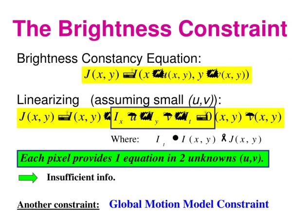
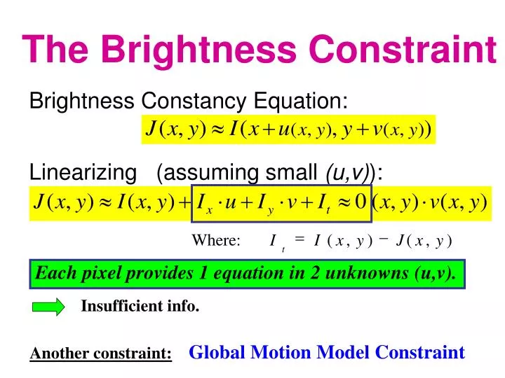
=. -. I. I. (. x. ,. y. ). J. (. x. ,. y. ). Where:. t. Insufficient info. The Brightness Constraint. Brightness Constancy Equation:. Linearizing (assuming small (u,v) ):. Each pixel provides 1 equation in 2 unknowns (u,v).

E N D
= - I I ( x , y ) J ( x , y ) Where: t Insufficient info. The Brightness Constraint Brightness Constancy Equation: Linearizing (assuming small (u,v)): Each pixel provides 1 equation in 2 unknowns (u,v). Another constraint:Global Motion Model Constraint
Requires prior model selection Camera motion + Scene structure + Independent motions The 2D/3D Dichotomy Camera induced motion = + Independent motions = Image motion = 2D techniques 3D techniques Do not model “3D scenes” Singularities in “2D scenes”
Global Motion Models 2D Models: • Affine • Quadratic • Homography (Planar projective transform) 3D Models: • Rotation, Translation, 1/Depth • Instantaneous camera motion models • Essential/Fundamental Matrix • Plane+Parallax
Least Square Minimization (over all pixels): Example: Affine Motion Substituting into the B.C. Equation: Each pixel provides 1 linear constraint in 6 global unknowns • (minimum 6 pixels necessary) Every pixel contributes Confidence-weighted regression
Example: Affine Motion Differentiating w.r.t. a1 , …, a6 and equating to zero 6 linear equations in 6 unknowns:
Coarse-to-Fine Estimation Jw refine warp + u=1.25 pixels u=2.5 pixels ==> small u and v ... u=5 pixels u=10 pixels image J image J image I image I Pyramid of image J Pyramid of image I Parameter propagation:
Quadratic– instantaneous approximation to planar motion Other 2D Motion Models Projective – exact planar motion (Homography H)
Generated Mosaic image Panoramic Mosaic Image Original video clip Alignment accuracy (between a pair of frames): error < 0.1 pixel
Video Removal Original Original Outliers Synthesized
Video Enhancement ORIGINAL ENHANCED
Direct Methods: Methods for motion and/or shape estimation, which recover the unknown parameters directly from measurable image quantities at each pixel in the image. Minimization step: Direct methods: Error measure based on dense measurable image quantities(Confidence-weighted regression; Exploits all available information) Feature-based methods: Error measure based on distances of a sparse set of distinct feature matches.
Example: The SIFT Descriptor • Compute gradient orientation histograms of several small windows (128 values for each point) • Normalize the descriptor to make it invariant to intensity change • To add Scale & Rotation invariance:Determine local scale (by maximizing DoG in scale and in space), local orientation as the dominant gradient direction. The descriptor(4x4 array of 8-bin histograms) Image gradients • Compute descriptors in each image Find descriptors matches across images Estimate transformation between the pair of images. • In case of multiple motions:Use RANSAC (Random Sampling and Consensus) to compute Affine-transformation / Homography / Essential-Matrix / etc. D.Lowe. “Distinctive Image Features from Scale-Invariant Keypoints”. IJCV 2004
Benefits of Direct Methods • High subpixel accuracy. • Simultaneously estimate matches + transformation Do not need distinct features. • Strong locking property.
Limitations • Limited search range (up to ~10% of the image size). • Brightness constancy assumption.
A camera-centric coordinate system (R,T,Z) Camera motion + Scene structure + Independent motions The 2D/3D Dichotomy Camera induced motion = + Independent motions = Image motion = 2D techniques 3D techniques Do not model “3D scenes” Singularities in “2D scenes”
The residual parallax lies on aradial (epipolar) field: epipole Original Sequence Plane-Stabilized Sequence The Plane+Parallax Decomposition
1. Reduces the search space: • Eliminates effects of rotation • Eliminates changes in camera parameters / zoom Benefits of the P+P Decomposition • Camera parameters: Need to estimate only epipole. • (gauge ambiguity: unknown scale of epipole) • Image displacements: Constrained to lie on radial lines • (1-D search problem) A result of aligning an existing structure in the image.
2. Scene-Centered Representation: Benefits of the P+P Decomposition Translation or pure rotation ??? Focus on relevant portion of info Remove global component which dilutes information !
2. Scene-Centered Representation: Shape =Fluctuations relative to a planar surface in the scene Benefits of the P+P Decomposition STAB_RUG SEQ
total distance [97..103] camera center scene global (100) component local [-3..+3] component 2. Scene-Centered Representation: Shape =Fluctuations relative to a planar surface in the scene Benefits of the P+P Decomposition • Height vs. Depth (e.g., obstacle avoidance) • Appropriate units for shape • A compact representation • - fewer bits, progressive encoding
3. Stratified 2D-3D Representation: • Start with 2D estimation (homography). Benefits of the P+P Decomposition • 3D info builds on top of 2D info. Avoids a-priori model selection.
Dense 3D Reconstruction(Plane+Parallax) Original sequence Plane-aligned sequence Recovered shape
Dense 3D Reconstruction(Plane+Parallax) Original sequence Plane-aligned sequence Recovered shape
Dense 3D Reconstruction(Plane+Parallax) Original sequence Plane-aligned sequence Recovered shape
p Epipolar line epipole Brightness Constancy constraint 1. Eliminating Aperture Problem P+P Correspondence Estimation The intersection of the two line constraints uniquely defines the displacement.
other epipolar line p Epipolar line another epipole epipole Brightness Constancy constraint 1. Eliminating Aperture Problem Multi-Frame vs. 2-Frame Estimation The other epipole resolves the ambiguity ! The two line constraints are parallel ==> do NOT intersect