Download
1 / 51
510 likes | 523 Views
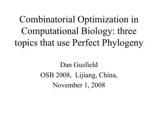
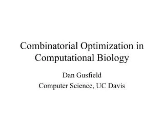
Combinatorial Algorithms and Optimization in Computational Biology and Bioinformatics. Dan Gusfield occbio, June 30, 2006. Two “Post-HGP” Topics. Two topics in Population Genomics SNP Haplotyping in populations Reconstructing a history of recombination

E N D
Combinatorial Algorithms and Optimization in Computational Biology and Bioinformatics Dan Gusfield occbio, June 30, 2006
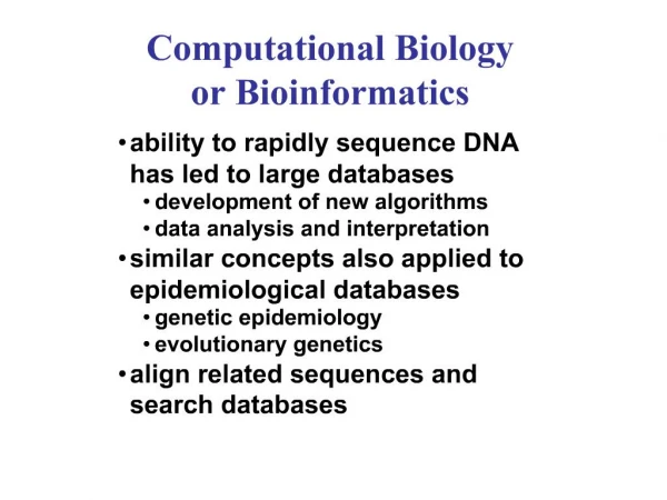
Two “Post-HGP” Topics Two topics in Population Genomics • SNP Haplotyping in populations • Reconstructing a history of recombination These topics in Population Genomics illustrate current challenges in biology, and illustrate the use of combinatorial algorithms and mathematics in biology.
What is population genomics? • The Human genome “sequence” is done. • Now we want to sequence many individuals in a population to correlate similarities and differences in their sequences with genetic traits (e.g. disease or disease susceptibility). • Presently, we can’t sequence large numbers of individuals, but we can sample the sequences at SNP sites.
SNP Data • A SNP is a Single Nucleotide Polymorphism - a site in the genome where two different nucleotides appear with sufficient frequency in the population (say each with 5% frequency or more). • SNP maps have been compiled with a density of about 1 site per 1000. • SNP data is what is mostly collected in populations - it is much cheaper to collect than full sequence data, and focuses on variation in the population, which is what is of interest.
Haplotype Map Project: HAPMAP • NIH lead project ($100M) to find common SNP haplotypes (“SNP sequences”) in the Human population. • Association mapping: HAPMAP used to try to associate genetic-influenced diseases with specific SNP haplotypes, to either find causal haplotypes, or to find the region near causal mutations. • The key to the logic of Association mapping is historical recombination in populations. Nature has done the experiments, now we try to make sense of the results.
Genotypes and Haplotypes Each individual has two “copies” of each chromosome. At each site, each chromosome has one of two alleles (states) denoted by 0 and 1 (motivated by SNPs) 0 1 1 1 0 0 1 1 0 1 1 0 1 0 0 1 0 0 Two haplotypes per individual Merge the haplotypes 2 1 2 1 0 0 1 2 0 Genotype for the individual
Haplotyping Problem • Biological Problem: For disease association studies, haplotype data is more valuable than genotype data, but haplotype data is hard to collect. Genotype data is easy to collect. • Computational Problem: Given a set of n genotypes, determine the original set of n haplotypepairs that generated the n genotypes. This is hopeless without a genetic model.
The Perfect Phylogeny Model for SNP sequences Only one mutation per site allowed. sites 12345 Ancestral sequence 00000 1 4 Site mutations on edges 3 00010 The tree derives the set M: 10100 10000 01011 01010 00010 2 10100 5 10000 01010 01011 Extant sequences at the leaves
When can a set of sequences be derived on a perfect phylogeny? Classic NASC: Arrange the sequences in a matrix. Then (with no duplicate columns), the sequences can be generated on a unique perfect phylogeny if and only if no two columns (sites) contain all four pairs: 0,0 and 0,1 and 1,0 and 1,1 This is the 4-Gamete Test
So, in the case of binary characters, if each pair of columns allows a tree, then the entire set of columns allows a tree. For M of dimension n by m, the existence of a perfect phylogeny for M can be tested in O(nm) time and a tree built in that time, if there is one. Gusfield, Networks 91 We will use the classic theorem in two more modern and more genetic applications.
The Perfect Phylogeny Model We assume that the evolution of extant haplotypes can be displayed on a rooted, directed tree, with the all-0 haplotype at the root, where each site changes from 0 to 1 on exactly one edge, and each extant haplotype is created by accumulating the changes on a path from the root to a leaf, where that haplotype is displayed. In other words, the extant haplotypes evolved along a perfect phylogeny with all-0 root. Justification: Haplotype Blocks, rare recombination, base problem whose solution to be modified to incorporate more biological complexity.
Perfect Phylogeny Haplotype (PPH) Given a set of genotypes S, find an explaining set of haplotypes that fits a perfect phylogeny. sites A haplotype pair explains a genotype if the merge of the haplotypes creates the genotype. Example: The merge of 0 1 and 1 0 explains 2 2. S Genotype matrix
The PPHProblem Given a set of genotypes, find an explaining set of haplotypes that fits a perfect phylogeny
The Haplotype PhylogenyProblem Given a set of genotypes, find an explaining set of haplotypes that fits a perfect phylogeny 00 1 2 b 00 a a b c c 01 01 10 10 10
The Alternative Explanation No tree possible for this explanation
Efficient Solutions to the PPH problem - n genotypes, m sites • Reduction to a graph realization problem (GPPH) - build on Bixby-Wagner or Fushishige solution to graph realization O(nm alpha(nm)) time. Gusfield, Recomb 02 • Reduction to graph realization - build on Tutte’s graph realization method O(nm^2) time. Chung, Gusfield 03 • Direct, from scratch combinatorial approach -O(nm^2) Bafna, Gusfield et al JCB 03 • Berkeley (EHK) approach - specialize the Tutte solution to the PPH problem - O(nm^2) time. • Linear-time solutions - Recomb 2005, and two other linear time solutions.
The Reduction Approach • This is the original polynomial time method from Recomb 2002.
The case of the 1’s • For any row i in S, the set of 1 entries in row i specify the exact set of mutations on the path from the root to the least common ancestor of the two leaves labeled i, in every perfect phylogeny for S. • The order of those 1 entries on the path is also the same in every perfect phylogeny for S, and is easy to determine by “leaf counting”.
In any column c, count two for each 1, and count one for each 2. The total is the number of leaves below mutation c, in every perfect phylogeny for S. So if we know the set of mutations on a path from the root, we know their order as well. Leaf Counting S Count 5 4 2 2 1 1 1
Simple Conclusions Subtree for row i data sites Root 1 2 3 4 5 6 7 i:0 1 0 1 222 The order is known for the red mutations together with the leftmost blue mutation. 2 4 5
But what to do with the remaining blue entries (2’s) in a row?
More Simple Tools • For any row i in S, and any column c, if S(i,c) is 2, then in every perfect phylogeny for S, the path between the two leaves labeled i, must contain the edge with mutation c. Further, every mutation c on the path between the two i leaves must be from such a column c.
From Row Data to Tree Constraints Subtree for row i data sites Root 1 2 3 4 5 6 7 i:0 1 0 1 222 2 4 Edges 5, 6 and 7 must be on the blue path, and 5 is already known to follow 4, but we don’t where to put 6 and 7. 5 i i
The Graph Theoretic Problem Given a genotype matrix S with n sites, and a red-blue subgraph for each row i, create a directed tree T where each integer from 1 to n labels exactly one edge, so that each subgraph is contained in T. i i
Powerfull Tool: Graph Realization • Let Rn be the integers 1 to n, and let P be an unordered subset of Rn. P is called a path set. • A tree T with n edges, where each is labeled with a unique integer of Rn, realizes P if there is a contiguous path in T labeled with the integers of P and no others. • Given a family P1, P2, P3…Pk of path sets, tree T realizes the family if it realizes each Pi. • The graph realization problem generalizes the consecutive ones problem, where T is a path.
Graph Realization Example 5 P1: 1, 5, 8 P2: 2, 4 P3: 1, 2, 5, 6 P4: 3, 6, 8 P5: 1, 5, 6, 7 1 8 6 2 4 3 7 Realizing Tree T
Graph Realization Polynomial time (almost linear-time) algorithms exist for the graph realization problem – Whitney, Tutte, Cunningham, Edmonds, Bixby, Wagner, Gavril, Tamari, Fushishige, Lofgren 1930’s - 1980’s Most of the literture on this problem is in the context of determining if a binary matroid is graphic. The algorithms are not simple; none implemented before 2002.
Reducing PPH to graph realization We solve any instance of the PPH problem by creating appropriate path sets, so that a solution to the resulting graph realization problem leads to a solution to the PPH problem instance. The key issue: How to encode the needed subgraph for each row, and glue them together at the root.
From Row Data to Tree Constraints Subtree for row i data sites Root 1 2 3 4 5 6 7 i:0 1 0 1 222 2 4 Edges 5, 6 and 7 must be on the blue path, and 5 is already known to follow 4. 5 i i
Encoding a Red-Blue directed path 2 P1: U, 2 P2: U, 2, 4 P3: 2, 4 P4: 2, 4, 5 P5: 4, 5 U 4 2 5 4 forced In T 5 U is a glue edge used to glue together the directed paths from the different rows.
Now add a path set for the blues in row i. sites Root 1 2 3 4 5 6 7 i:0 1 0 1 222 2 4 5 P: 5, 6, 7 i i
That’s the Reduction The resulting path-sets encode everything that is known about row i in the input. The family of path-sets are input to the graph- realization problem, and every solution to the that graph-realization problem specifies a solution to the PPH problem, and conversely. Whitney (1933?) characterized the set of all solutions to graph realization (based on the three-connected components of a graph) and Tarjan et al showed how to find these in linear time.
Combinatorial Algorithms for estimating and reconstructing recombination in populations Dan Gusfield UC Davis Different parts of this work are joint with Satish Eddhu, Charles Langley, Dean Hickerson, Yun Song, Yufeng Wu, Z. Ding OCCBIO June 29, 2006
A richer model 10100 10000 01011 01010 00010 10101 added 12345 00000 1 4 M 3 00010 2 10100 5 Pair 4, 5 fails the four gamete-test. The sites 4, 5 ``conflict”. 10000 01010 01011 Real sequence histories often involve recombination.
Sequence Recombination 01011 10100 S P 5 Single crossover recombination 10101 A recombination of P and S at recombination point 5. The first 4 sites come from P (Prefix) and the sites from 5 onward come from S (Suffix).
Network with Recombination 10100 10000 01011 01010 00010 10101 new 12345 00000 1 4 M 3 00010 2 10100 5 P 10000 01010 The previous tree with one recombination event now derives all the sequences. 01011 5 S 10101
A Phylogenetic Network or ARG 00000 4 00010 a:00010 3 1 10010 00100 5 00101 2 01100 S b:10010 P S 4 01101 c:00100 p g:00101 3 d:10100 f:01101 e:01100
A tree-like network for the same sequences generated by the prior network. 4 3 1 s p a: 00010 2 c: 00100 b: 10010 d: 10100 2 5 s p 4 g: 00101 e: 01100 f: 01101
Recombination Cycles • In a Phylogenetic Network, with a recombination node x, if we trace two paths backwards from x, then the paths will eventually meet. • The cycle specified by those two paths is called a ``recombination cycle”.
Galled-Trees • A phylogenetic network where no recombination cycles share an edge is called a galled tree. • A cycle in a galled-tree is called a gall. • Question: if M cannot be generated on a true tree, can it be generated on a galled-tree?
Results about galled-trees • Theorem: Efficient (provably polynomial-time) algorithm to determine whether or not any sequence set M can be derived on a galled-tree. • Theorem: A galled-tree (if one exists) produced by the algorithm minimizes the number of recombinations used over all possible phylogenetic-networks. • Theorem: If M can be derived on a galled tree, then the Galled-Tree is ``nearly unique”. This is important for biological conclusions derived from the galled-tree. Papers from 2003-2005.
Elaboration on Near Uniqueness Theorem: The number of arrangements (permutations) of the sites on any gall is at most three, and this happens only if the gall has two sites. If the gall has more than two sites, then the number of arrangements is at most two. If the gall has four or more sites, with at least two sites on each side of the recombination point (not the side of the gall) then the arrangement is forced and unique. Theorem: All other features of the galled-trees for M are invariant.
Incompatible Sites A pair of sites (columns) of M that fail the 4-gametes test are said to be incompatible. A site that is not in such a pair is compatible.
1 2 3 4 5 Incompatibility Graph G(M) a b c d e f g 0 0 0 1 0 1 0 0 1 0 0 0 1 0 0 1 0 1 0 0 0 1 1 0 0 0 1 1 0 1 0 0 1 0 1 4 M 1 3 2 5 Two nodes are connected iff the pair of sites are incompatible, i.e, fail the 4-gamete test. THE MAIN TOOL: We represent the pairwise incompatibilities in a incompatibility graph.
The connected components of G(M) are very informative • Theorem: The number of non-trivial connected components is a lower-bound on the number of recombinations needed in any network. • Theorem: When M can be derived on agalled-tree, all the incompatible sites in a gall must come from a single connected component C, and that gall must contain all the sites from C. Compatible sites need not be inside any blob. • In a galled-tree the number of recombinations is exactly the number of connected components in G(M), and hence is minimum over all possible phylogenetic networks for M.
Incompatibility Graph 4 4 3 1 3 2 5 1 s p a: 00010 2 c: 00100 b: 10010 d: 10100 2 5 s p 4 g: 00101 e: 01100 f: 01101
Efficient Algorithm The connected components of the conflict graph are the key to efficiently determining if the sequences can be derived on a galled-tree, and to construct one if possible.
Coming full circle - back to genotypes When can a set of genotypes be explained by a set of haplotypes that derived on a galled-tree, rather than on a perfect phylogeny? Recently, we developed an Integer Linear Programming solution to this problem, and are now testing the practical efficiency of it. (Brown, Gusfield 2006).