Download

1 / 42
440 likes | 837 Views
Matrices. Student Handbook. Matrices. A matrix (plural: matrices , not matrixes) is a rectangular array of numbers such as Matrices are useful when modelling a variety of real-life problems , and are the abstract mathematical counterparts of array data structures in programming.

E N D
Matrices Student Handbook
Matrices • A matrix (plural: matrices, not matrixes) is a rectangular array of numbers such as • Matrices are useful when modelling a variety of real-life problems, and are the abstract mathematical counterparts of array data structures in programming.
Matrix Entries • In this section we show how to add and multiply matrices. • We shall identify the numbers inside a matrix by their position. In matrix A = • we may describe the number 1 as “the entry in the firstrow, firstcolumn”, or more precisely write a11 = 1.
Matrix Entries • Similarly a12 = 2 is the entry in the first row, second column. • More generally we write aijfor the entry in the ithrow, jthcolumn. • Matrices come in different sizes. Since A has two rows and three columns, we call A a 2×3 or “2by3” matrix. • The size of a matrix determines what other matrices it can be added to or multiplied with. • Matrices are equal if they are the same size and their corresponding entries are equal.
Addition • Two matrices A and B of the same size can be added together and the sum A+B is obtained by adding the corresponding entries. • For example
Addition • However, the sum is not defined, since the first matrix is 3×2 but the second is 3 × 3.
Scalar Multiplication • To multiply a matrixA by a scalarc just means that c is some real number and that we multiply every entry in Abyc. • Let A = and let c = , then
Scalar Multiplication • The differenceA - B of two matrices of the same size is just another way of writing A + (-1)B:
Matrix Multiplication • If A is a k × m matrix and B is an m × n matrix, then the productC = AB is the k×n matrix whose entries are found as follows: • To calculate cij, take rowi from matrix A and columnj from matrix B, multiply the corresponding entries together, and add up the results. • Note that AB is defined iff the number of columns of A matches the number of rows of B.
Matrix Multiplication • For example is undefined, because the matrices to be multiplied are 3 × 2 and 3 × 2. • So it is possible to have two matrices that can be added but not multiplied together.
Examples of Products where the matrices to be multiplied are 1 × 2 and 2 × 1, so that multiplication is defined and the product is 1 × 1.
Examples of Products where the matrices to be multiplied are 3 × 2 and 2 × 2, so that multiplication is defined and the product is 3 × 2.
Why? • Let’s show, by a real-life example, why matrix multiplication is defined in such a strange way. • Suppose a superannuation fund has investments in three countries. • The deposits in each country are divided among government bonds, mortgages, and shares. • Let’s represent the amount currently invested in each country, in millions of dollars, by the table
Why? BondsMortgages Shares Country A 5 10 20 Country B 3 9 15 Country C 2 6 10 • The table can be simplified to the matrix X =
Why? • Now suppose the average yields are 4% for bonds, 7% for mortgages, and 10% for shares. • How would we work out the earnings the superannuation fund can expect from its investments in each country?
Why? • The amount earned in Country A would be (amount invested in bonds)·(yield of bonds) + (amount in mortgages) ·(yield of mortgages) + (amount in shares) ·(yield of shares) = (5)(.04) + (10)(.07) + (20)(.10). • This is like working out an entry in a matrix product.
Why? • Let the yield matrix be Y = • Then the amount earned in CountryA is just the first entry of the product XY =
Why? • and the earnings for the other countries are the second and third entries: • The fund earns 2.9 million in CountryA, 2.25 million in CountryB, and 1.5 million in CountryC.
Representing Systems of Equations • Here is another use for products. The system of linear equations 2x - 3y = 5 4x + y = 0 can be represented compactly by the matrix equation:
Representing Systems of Equations which is of the form AX = B where
A Real Life Problem • You have a bacteria culture containing three species of bacteria. Each species requires different amounts of threenutrients: nitrates, carbohydrates, and phosphates. • The requirements are given in the table, in micrograms per day. SpeciesNitratesCarbohydratesPhosphates A 1 2 1 B 2 3 1 C 3 2 2
A Real Life Problem • The daily supply of nitrates is 6000 units, of carbohydrates is 7000 units, and of phosphates is 4000 units. • How many bacteria of each species can the culture grow?
Modelling the data • Let x be the number of bacteria of species A, y the number of B, and z the number of C. • We want to use our data to find the values of x, y, and z. • But first we have to represent that data in a way that connectsthe information with the unknownsx, y, and z. • This gives us a system of linear equations:
Modelling the data • If the entire daily supply of 6000 units of nitrates is used up, then x + 2y + 3z = 6000. • Similarly, from the data about carbohydrates we get 2x + 3y + 2z = 7000 • and from the phosphate data we get x + y + 2z = 4000.
Solving Linear Equations • In this section we show how matrices arise when solving systems of linear equations. • Key concepts in this section: system of linear equations, augmented matrix, coefficient matrix, elementary transformation, echelon form, rank of a matrix.
Echelon Form • We have the following system of equations to solve: x + 2y + 3z = 6000 2x + 3y + 2z = 7000 x + y + 2z = 4000 • but it is unclear what values of x, y, and z would satisfy the equations.
Echelon Form • So we transform this system into a new system which has the same solutions but is easier to solve. • If the new system is in echelon form it is easy to solve: x + 2y + 3z = 6000 y + 4z = 5000 3z = 3000 • Now z = 1000 and back-substituting gives y = 5000-4000 = 1000 and x = 6000-2000-3000 =1000.
Matrix Representation • Suppose we are going to transform the system of equations into a new system in echelon form. • It will reduce the labour if we simplify the representation. • Instead of writing down the equations, we write down just the coefficients of the unknowns on the left and the constants on the right, giving us the augmented matrix of the system.
Matrix Representation • So from the system x + 2y + 3z = 6000 2x + 3y + 2z = 7000 x + y + 2z = 4000 • we get the augmented matrix
Elementary Transformations We can change a system of equations into a new system with the same solutions: • by swapping equations or • by multiplying through by a nonzero number or • by adding one equation to another. • In terms of the augmented matrix, this means we may:
Elementary Transformations • interchange two rows: Rj↔ Rk • multiply through by a nonzero number: Rj⟶ c × Rj • add one row to another row: Rj⟶ Rj + Rk. • In fact, we often combine the last two transformations so as to add a multiple of one row to another row: • Rj⟶ Rj + c × Rk
Example • The system of linear equations gives • R2⟶ R2 - 2R1and then R3⟶ R3 - R1 give
Example • R2⟶ (-1) R2and then R3⟶ R3 + R2give • This matrix represents the system of equations x + 2y + 3z = 6000 y + 4z = 5000 3z = 3000
Example with solutionsx = 1000, y = 1000, and z = 1000. • By using elementary transformations to reduce the augmented matrix to echelon form. • We get a new system of equations with the same solutions as the original system. • The technique is called Gaussian elimination.
No Solutions? • When the augmented matrix of a system of linear equations in n unknowns is reduced to echelonform, the last row may be of the form [0 … 0 c]with c ≠ 0 • so that the corresponding equation is 0 x1 + …+ 0 xn = c • which has no solution, because no matter what values we substitute for the unknowns x1, x2, …, xn
No Solutions? • The lefthand side still adds up to zero, whereas the righthand side is nonzero. • But if the last row has at least one nonzero coefficient [0 …an c]where an≠ 0 • Then the system has at least one solution, irrespective of the value of c, since the final equation is 0x1 + …+ anxn = c
Infinitely Many Solutions • Suppose our model was initially the system x + 2y + 3z = 6000 2x + 3y + 2z = 7000 • which we reduced to echelon form to get x + 2y + 3z = 6000 y + 4z = 5000
Infinitely Many Solutions • Instead of a unique value for z, we can let z be any real numbert, and then get values for y and x in terms of t, namely y = 5000 - 4t and x = 6000 - 2(5000 - 4t) - 3t = 5t - 4000. • We can produce specific solutions by giving t specific values such as t = 0 (so that x = -4000, y = 5000, and z = 0) and t = 1 (so that x = -3995, y = 4996, and z = 1).
Homogeneous Systems • If the constants on the righthand side are all zero, as in the system x + 2y + 3z = 0 2x + 3y + 2z = 0 x + y + 2z = 0 then the system always has at least one solution, because we may take x = y = z = 0. • Such systems of equations are called homogeneous.
Homogeneous Systems • We need not use an augmented matrix to represent a homogeneous system, since the last column will consist entirely of zeros. • Instead we may use the coefficient matrix in which only the values of the coefficients of the unknowns are displayed:
Rank • The rank of a matrix is the number of nonzero rows left after the matrix has been reduced to echelon form. • A system of linear equations has a solution iff the rank of the augmented matrix is equal to the rank of the coefficient matrix. • Why?
Rank • Because the only way for a system to have no solutions is for the augmented matrix in echelon form to have as its last nonzero row [0 … 0c] with c ≠ 0. • But now the rank of the augmented matrix is greater than the rank of the coefficient matrix. • So if the ranks are equal, it means that this case cannot arise

![[MATRICES ]](https://cdn4.slideserve.com/144276/matrices-dt.jpg)