Download
1 / 59
590 likes | 734 Views
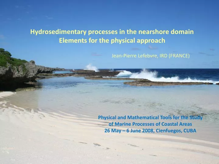
Hydrosedimentary processes in the nearshore domain Elements for the physical approach. Jean-Pierre Lefebvre, IRD (FRANCE). Physical and Mathematical Tools for the Study of Marine Processes of Coastal Areas 26 May – 6 June 2008, Cienfuegos, CUBA. Erosion, suspension, fluidization. FORCING.

E N D
Hydrosedimentary processes in the nearshore domainElements for the physical approach Jean-Pierre Lefebvre, IRD (FRANCE) Physical and Mathematical Tools for the Study of Marine Processes of Coastal Areas 26 May – 6 June 2008, Cienfuegos, CUBA
Erosion, suspension, fluidization FORCING SEABEDS Permanent stress (current) Non cohesive sediment (sand) Oscillatory stress (wave) Cohesive sediment (mud) Turbulence, energy dissipation, shoaling
FORCINGS I. Permanent flow II. Oscillatory flow SEDIMENTS III. Cohesive sediments
Permanent flow (laminar) z u(z) Newton’s law of viscosity boundary layer : for a viscous flow, layer defined from the bed (non slip condition) up to the height where the flow is no longer perturbed by the wall. µ : (absolute) dynamic viscosity (Pa.s) (1.08 10−3 Pa.s for seawater at T = 20°C and S = 35 g.kg-1) n: kinematic fluid viscosity (m².s-1) rw: density of water (kg.m-3) (≈ 1.025 for seawater for T =20°C, S = 35 g.kg-1)
time averaged (steady) component Permanent flow (turbulent) turbulent flow : fluid regime characterized by chaotic property changes. This includes high frequenty variation of velocity in space and time. u’(t,z) u(t,z) Reynolds decomposition of a parameter t 0 T t 0 T _ fluctuating component (perturbation) Instantaneous local velocity steady component da Vinci sketch of a turbulent flow
Permanent flow (turbulent) Turbulent shear stress ne: kinematic eddy viscosity (m².s-1) Reynolds stress tensor (covariance of vertical and horizontal velocities)
Permanent flow (turbulent) Turbulent boundary layer h OUTER REGION ∿ 0.1h LOG LAYER VISCOUS SUB-LAYER δv • Turbulent outer region • influenced by the outer boundary condition of the layer, • consists of about 80-90 % of the total region, • velocity relatively constant due to the strong mixing of the flow. • Intermediate region (log layer) • logarithmic profile of the horizontal velocity • Innermost region (viscous sub layer) • dominated by viscosity, • linear velocity profile , • very small.
Permanent flow (turbulent) The characteristic velocity scale u* is a parameter of the order of magnitude of the turbulent velocity often called friction velocity since it is used as the actual turbulent velocity action on the bed z Friction velocity ∿ 0.1h LOG LAYER δv VISCOUS SUB LAYER u
Permanent flow (turbulent) Prandtl’s model of mixing-length in the turbulent boundary layer, states that the turbulence is linearly related to the averaged velocity gradient by a term Lm called, mixing length z - ∿ 0.1h LOG LAYER von Kármán assumption states that the correlation scale is proportional to the distance from the boundary δv VISCOUS SUB LAYER u von Kármán constant (κ = 0.408 ) the kinematic eddy viscosity must also be proportional to the height above the bed.
Permanent flow (turbulent) z Prandtl-Kármán law of wall ∿ 0.1h LOG LAYER δv VISCOUS SUB LAYER z0 : hydraulic roughness of the flow depends on viscous sub-layer, grain roughness, ripples and other bedforms, stratification,… u
Permanent flow (turbulent) z Nikuradse sand roughness (physical roughness) can be approximated by the median diameter of grains of sandy bed ∿ 0.1h LOG LAYER δv VISCOUS SUB LAYER u d50 : mean particles diameter
Permanent flow (turbulent) the viscous sub-layer is a narrow layer close to the wall where roughness of the wall and molecular viscosity dominate transport of momentum z ∿ 0.1h LOG LAYER Ratio of inertial force to viscous force δv VISCOUS SUB LAYER Thickness of the viscous sub-layer u
Permanent flow (turbulent) The relative roughness (ratio of hydraulic roughness z0 on the physical roughness ks) depends on the relative length scales for the viscous sub-layer and the physical roughness roughness Reynolds or grain Reynolds number
Rough regime Permanent flow (turbulent) • Hydraulically rough regime : Re* > 70 • the viscous sub-layer is interrupted by the bed roughness, • roughness elements interact directly with the turbulence.
Permanent flow (turbulent) Hydraulically smooth regime : Re* < 5 the viscous sub-layer lubricates the roughness elements so they do not interact with turbulence. Smooth regime Rough regime
+ Permanent flow (turbulent) hydraulically transitional regime : 5 ≤ Re* ≤ 70 For 0.26 < ks/v < 8.62 the near-wall flow is transitional between the hydraulically smooth and hydraulically rough regimes Smooth regime Transitional regime Rough regime
Permanent flow (turbulent) Bottom shear stress turbulent outer layer friction factor log layer Friction factor for current (rough turbulent regime) transition layer viscous sub-layer
Permanent flow (turbulent) Measurements Quantification Description Velocities at some elevations near the bed Sediment granular distribution Friction velocity and hydraulic roughness Physical roughness Turbulent shear stress at the bed Hydraulic turbulent regime FORCING SEABEDS Prandtl-Kármán law of wall Nikuradse approximation
Oscillatory flow • Waves can be defined by their superficial properties • wave height (distance between its trough and crest) • wave length (distance between two crests) • wave period (duration for the propagation of two successive extrema at a given location) wave height (m) wave amplitude (m) angular velocity (rad.s-1) wave period (s) wave number (rad.m-1) wavelength (m)
Oscillatory flow Airy wave : model for monochromatic progressive sinusoidal waves Wave with multispectral components
Oscillatory flow velocity potential ∅ • Assuming an oscillatory flow V of an inviscid , incompressible fluid, • with no other motions interfering (i.e. no currents) • irrotational flow (i.e. no curl between the water particles trajectories) : V = 0 • satisfying the continuity equation : . V = 0 • For a sinusoidal wave field, it exists an ideal potential flow solution: ∅ = V • from which we can derivate the expressions of all the pressure and flow fields.
Oscillatory flow Equation of Laplace for the inviscid, uncompressible flow BOUNDARY CONDITIONS Kinematic boundary condition : a parcel of fluid at the surface remains at the surface Dynamic boundary condition : the pressure along an iso-potential line is constant (Bernoulli ) Boundary condition : the bottom is not permeable to water
Oscillatory flow For small amplitude gravity wave (wave amplitude a << wavelength λ)
Oscillatory flow Linearization (only the first order terms of the Taylor series) Laplacian equation SIMPLIFIED BOUNDARY CONDITIONS Simplified Kinematic boundary condition Simplified dynamic boundary condition Simplified boundary condition
Oscillatory flow General form of ∅ for a sinusoidal wave
Oscillatory flow SURFACE ELEVATION From = -gη at z = 0 VELOCITY FIELD from ∅ = V PRESSURE From p = -ρw ∂∅ ∂∅ ___ ___ ∂t ∂t
Oscillatory flow DISPERSION EQUATION The relation between the angular velocity ω and the wave number (from the simplified Laplace equation) WAVE CELERITY velocity of the wave crest ( m.s-1)
Oscillatory flow DISPERSION EQUATION DEEP WATER DOMAIN The water height is much greater than the wavelength (h >> λ) WAVE CELERITY
Oscillatory flow DISPERSION EQUATION WAVE CELERITY SHALLOW WATER DOMAIN The wavelength is much greater than the water height (λ >>h)
Oscillatory flow INTERMEDIATE DOMAIN
Oscillatory flow Wave breaking shoaling SWL Limit of lower orbital motions Strong erosion Slight erosion of the seabed No erosion of the seabed SHALLOW WATER INTERMEDIATE ZONE DEEP WATER λ λ __ __ h h 20 2 ∿ ∿
Oscillatory flow Orbital velocity at the bed Stokes’ drift
Oscillatory flow (turbulent) Wave boundary layer thickness maximum shear velocity Turbulent wave shear stress
Oscillatory flow (turbulent) Law of wall (Grant and Madsen) Phase lead
Oscillatory flow (turbulent) Shear stress generated by the oscillatory flow where
Oscillatory flow (turbulent) Maximum shear stress friction factor for wave Friction factor for wave (rough turbulent regime)
Oscillatory flow (turbulent) Measurements Description Quantification Surface wave parameters and wave height Sediment granular distribution Maximum shear velocity and hydraulic roughness Physical roughness Maximum shear stress at the bed Hydraulic turbulent regime SEABEDS FORCING Grant-Madsen Law of wall Nikuradse approximation
Oscillatory flow Potential Energy Kinetic Energy Energy density (J.m-2)
Oscillatory flow Flux of energy (J) Group Velocity (m.s-1) In deep water domain (kh→∞) and Cg = C/2 In shallow water domain (kh→0) and Cg = C
Oscillatory flow Shoaling Wave period : 8 s Wave height (m) ∿ 2.3 hdw= 49.6 m hsw= 0.8 H __ 0.8 h Water depth (m) 2.8
Combined current and wave stresses many empirical expressions exist for coupling permanent and oscillatory stresses (Soulsby, 1995)
seabed Transport mode for marine sediments Bed-load transport The rolling, sliding and jumping grains in almost continuous contact with the bed. Intergranular collision forces play an important role Suspended-load transport Grains are almost continuously suspended in the water column The turbulence mixing processes are dominant Sheet flow a layer with a thickness of several grain layers (10–100) and large sediment concentrations is transported along the bed.
seabed Sediment cohesion : domination of interparticle forces or the gravitational force in the behavior of sediment. Cohesive sediments : material with strong interparticle forces due to their surface ionic charges Non cohesive sediments : granular material dominated by the gravitational force GRAVEL CLAY SILT SAND COBBLES gravel cobbles clay pea gravel very fine very coarse very fine very coarse fine medium coarse medium coarse fine medium coarse 2µ 4 8 16 32 64 125 250 500 1mm 2 4 8 16 32 64
Erosion critical shear stress fully controled flow (flow, chenal dimensions, fixed bottom roughness) Suspended fine sediments measured with OBS Erosion and transport ( bedload and suspension) Non cohesive sediment trapping (gravitation) Measurements of the erosion (erodimeter, IFREMER) In situ sampling of unperturbed seabed extractionof the unperturbed interface Grain size spectrum of defloculated material
Flocculation Mud flocs are characterized by four main physical properties: • size (diameter) Df • density ρfloc • settling velocity Ws • floc strength Fc Mud floc properties are governed by four mechanisms: • Brownian motions cause the particles to collide to form aggregates • particles with a large settling velocity will overtake particles with a low settling velocity and aggregate • turbulent motions will cause particles, carried by the eddies • to collide and form flocs • turbulent shear may disrupt the flocs again, causing floc breakup
Flocculation Self similarity clay < 4µm fine silt (4 ∿ 10µm) flocculus Microfloc (< 100µm) microfloc Macrofloc ( ∿O(2) µm up to ∿ O(1) mm) flocculus strong bound by sticky material produced by biological organisms strong interparticle forces due to surface ionic charges loosely bound and very fragile
Flocculation Floc size The fractal dimension nf is obtained from the description of a growing object with linear size αL and volume V(αL) α ( linear size of the primary object (seed) (arbitrary = 1) number of seeds in estuarine and coastal environments 1.7 < nfloc < 2.2
Flocculation Floc excess density defloculated particles diameter floc diameter Sediment density ρsfor clay ∿ 1390 kg.m-3
Flocculation Floc limitation by turbulence the energy dissipation rate per unit mass ε expresses the process of energy transfer the cut-off floc diameter is determined by the local balance of floc growth and rupture within a turbulent fluid regime. volume average value of ε (J) Rate of turbulent shear