Download
1 / 67
680 likes | 825 Views
Figure 11.1 State variable compensator employing full-state feedback in series with a full-state observer. Figure 11.2 Third-order system. (a) Signal-flow graph model. (b) Block diagram model. Figure 11.3 (a) Flow graph model for Example 11.2. (b) Block diagram model.

E N D
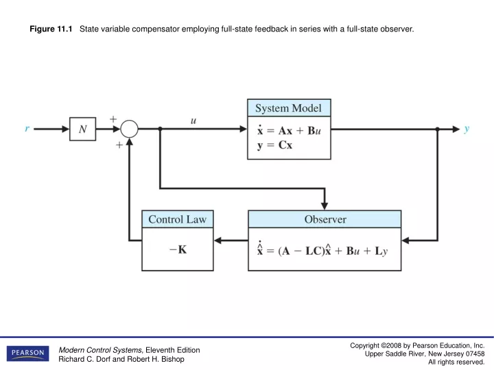
Figure 11.1 State variable compensator employing full-state feedback in series with a full-state observer.
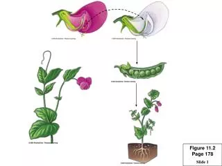
Figure 11.2 Third-order system. (a) Signal-flow graph model. (b) Block diagram model.
Figure 11.3 (a) Flow graph model for Example 11.2. (b) Block diagram model.
Figure 11.4 Two state system model for Example 11.4. (a) Signal-flow graph model. (b) Block diagram model.
Figure 11.5 Full-state feedback block diagram (with no reference input).
Figure 11.7 Second-order observer response to initial estimation errors.
Figure 11.8 State variable compensator with integrated full-state feedback and observer.
Figure 11.9 System pole map: open-loop poles, desired closed-loop poles, and observer poles.
Figure 11.10 Pendulum performance under full-state feedback control with the observer in the loop.
Figure 11.11 State variable compensator with a reference input.
Figure 11.12 State variable compensator with reference input and M = BN.
Figure 11.13 State variable compensator with reference input and N = 0 and M = -L.
Figure 11.18 Performance index versus the feedback gain k for Example 11.12.
Figure 11.19 Performance index versus the feedback gain k for Example 11.13.
Figure 11.21 Internal model design response to an initial tracking error for a unit step input.
Figure 11.22 Internal model design for a ramp input. Note that G(s)Gc(s) contains 1/s2, the reference input R(s).
Figure 11.25 Open-loop block diagram of the DC motor with mounted encoder wheel.
Figure 11.30 Elements of the control system design process emphasized in this diesel electric locomotive example.
Figure 11.31 Signal flow graph of the diesel electric locomotive. (a) Signal flow graph. (b) Block diagram controller feedback loops are shown in light.
Figure 11.32 Block diagram representation of the diesel electric locomotive.
Figure 11.33 Desired location of the closed-loop poles (that is, the eigenvalues of A - BK).
Figure 11.34 Closed-loop step response of the diesel electric locomotive.
Figure 11.37 Controllability with radial thrusters only: (a) m-file script, (b) output.
Figure 11.38 Controllability with tangential thrusters only: (a) m-file script, (b) output.
Figure 11.39 (a) Root locus for the automatic test system. (b) m-file script.
Figure 11.42 Using acker to compute K to place the poles at P = [-1 + j -1 - j]Ƭ.
Figure 11.44 Closed-loop system with feedback of the two state variables.
Figure E11.11 State variable block diagram with a feedforward term.
Figure P11.9 (a) Ball and beam. (b) Model of the ball and beam.