Download
1 / 41
410 likes | 496 Views
Prediction concerning Y variable. Three different research questions. What is the mean response , E(Y h ), for a given level, X h , of the predictor variable? What would one predict a new observation , Y h(new) , to be for a given level, X h , of the predictor variable?

E N D
Three different research questions • What is the mean response, E(Yh), for a given level, Xh, of the predictor variable? • What would one predict anew observation, Yh(new) , to be for a given level, Xh, of the predictor variable? • What would one predict themean of m new observations, , to be for a given level, Xh, of the predictor variable?
Example: Mortality and Latitude • What is the expected (mean) mortality rate for locations at 40o N latitude? • What is the predicted mortality rate for a new randomly selected location at 40o N? • What is the predicted mortality rate for 10 new randomly selected locations at 40o N?
is the best point estimator in each case. Point estimators • That is, it is: • the best guess of the mean response at Xh • the best guess of a new observation at Xh • the best guess of a mean of m new observations at Xh But, as always, to be confident in the answer to our research question, we should put an interval around our best guess.
Y-hat-h is normally distributed Sampling distribution of Y-hat-h Providing error terms εi are normally distributed: with mean E(Yh) and variance
Implications on precision • The greater the spread in the Xi values, the smaller the variance of Y-hat-h, the more precise the prediction of E(Yh). • Given the same set of Xi values, the further Xh is from the (sample) mean of the Xi, the greater the variance of Y-hat-h, the less precise the prediction of E(Yh).
Estimate of the variance Estimate variance with Then, the estimated standard deviation is
Confidence interval for E(Yh) Sample estimate ± margin of error
The estimation in Minitab • Stat >> Regression >> Regression … • Specify response and predictor(s). • Select Options… In “Prediction intervals for new observations” box, specify either the X value or a column name containing multiple X values. Specify confidence level. • Click on OK. Click on OK. • Results appear in session window.
Predicted Values for New Observations New Fit SE Fit95.0% CI 95.0% PI 1 150.08 2.75(144.6,155.6) (111.2,188.93) 2 221.82 7.42(206.9,236.8) (180.6,263.07)X X denotes a row with X values away from the center Values of Predictors for New Observations New Obs Latitude 1 40.0 2 28.0
“Fit” is “SE Fit” is Therefore, the “95% CI” for E(Yh) is Minitab output
Difference in precision of estimates • The mean of the 49 latitudes in the data set is 39.5o N. • SE Fit for Xh=40 is 2.75. • SE Fit for Xh=28 is 7.42 (larger as expected). • The closer Xh is to the sample mean, the narrower the confidence interval, the more precise the estimate of E(Yh).
Comments on assumptions • Xh is value within scope of model, that is, within range of X values in data set, but not necessary that it is one of the X values. • It is OK to use the formula for the confidence interval for E(Yh) even if the error terms are only approximately normally distributed. • If you have a large sample, the error terms can even deviate substantially from normality without greatly affecting appropriateness of the confidence interval.
Restatement of problem • We previously estimated the mean response E(Yh). That is, we estimated the mean of the distribution of Y at a given Xh. • Now, we want to predict a new response Yh(new). That is, we predict an individual outcome Y at a given Xh. • Most outcomes Y deviate from the mean response E(Yh). We must take this into account when we predict Yh(new).
How to obtain a prediction interval if distribution of Y is known • If you know the distribution of Y, you know • its shape (say, it’s normal) • its mean (say, it’s μ (“mu”)) • its standard deviation (say, it’s σ (“sigma”)) • BASIC IDEA: Using the distribution, determine a range in which most of the Y observations will fall. Claim that the next observation will fall there, too.
Example: High school GPA (X) and College GPA (Y) • Distribution of college GPA (Y) depends on high school GPA (X) through intercept and slope parameters. • Suppose: • Y is normally distributed • Mean is E(Y) = 0.10 + 0.95 X • Standard deviation σ (“Sigma”) = 0.12 • For students with X = 3.5 high school GPA: • E(Y) = 0.10 + 0.95(3.5) = 3.425
Example: 99.7% prediction interval for Yh(new) • The probability that a randomly selected high school student with a GPA of 3.5 will have a college GPA between • 3.425 - 3(0.12) = 3.065 and • 3.425 + 3(0.12) = 3.785 is 0.997.
But we have a problem … • The last calculation was possible because we knew β0, β1, and σ. Hence, we knew the mean and variance, E(Y) and σ2, respectively, of the distribution of Y. • We could consider estimating E(Y) and σ2 with Y-hat-h and MSE, respectively, and applying the same method as before. • But, it’s not quite right. Here’s why.
So … • We cannot be certain of the location (mean) of the distribution of Y. • Prediction limits for Yh(new) must take into account: • variation in possible location (mean) of the distribution of Y • variation in the Y of the probability distribution
Variation of the prediction The variation in the prediction of a new response depends on two components: the variation due to estimating E(Yh) with Y-hat-h and the variation in Y within the probability distribution. which is estimated by:
Prediction interval for Yh(new) Providing error terms εi are normally distributed:
The prediction in Minitab • Stat >> Regression >> Regression … • Specify response and predictor(s). • Select Options… In “Prediction intervals for new observations” box, specify either the X value or a column name containing multiple X values. Specify confidence level. • Click on OK. Click on OK. • Results appear in session window.
S = 19.12 R-Sq = 68.0% R-Sq(adj)= 67.3% Predicted Values for New Observations New Fit SE Fit95.0% CI 95.0% PI 1 150.08 2.75 (144.6,155.6) (111.2,188.93) 2 221.82 7.42 (206.9,236.8) (180.6,263.07)X X denotes a row with X values away from the center Values of Predictors for New Observations New Obs Latitude 1 40.0 2 28.0
“Fit” is Therefore, the “95% PI” for Yh(new) is Minitab output
As always, some comments… • In general, prediction intervals are wider than confidence intervals. • Prediction intervals are (somewhat) wider the further Xh is from the mean of the X values. • The formula for the prediction interval depends strongly on the assumption that the error terms are normally distributed.
Remember the distinction … • A confidence interval concerns the estimation of an unknown parameter. It is an interval that is intended to cover the value of the unknown parameter. • A prediction interval, on the other hand, is a statement about the value to be taken by a random variable, here, the new observation Yh(new).
Getting a plot of the CI and PI in Minitab • Stat >> Regression >> Fitted line plot … • Specify predictor and response. • Under Options …Select Display confidence bands. Select Display prediction bands. Specify desired confidence level. • Select OK. Select OK.
Row Xh Xbar sumsqX n MSE SD_EY SD_Pred 1 28 39.533 1020.54 49 365.383 7.42147 20.5052 2 29 39.533 1020.54 49 365.383 6.86862 20.3116 3 30 39.533 1020.54 49 365.383 6.32406 20.1340 4 31 39.533 1020.54 49 365.383 5.79013 19.9727 5 32 39.533 1020.54 49 365.383 5.27006 19.8282 6 33 39.533 1020.54 49 365.383 4.76838 19.7008 7 34 39.533 1020.54 49 365.383 4.29156 19.5908 8 35 39.533 1020.54 49 365.383 3.84884 19.4986 9 36 39.533 1020.54 49 365.383 3.45337 19.4244 10 37 39.533 1020.54 49 365.383 3.12313 19.3685 11 38 39.533 1020.54 49 365.383 2.88066 19.3308 12 39 39.533 1020.54 49 365.383 2.74927 19.3117 13 40 39.533 1020.54 49 365.383 2.74497 19.3111 14 41 39.533 1020.54 49 365.383 2.86833 19.3290 15 42 39.533 1020.54 49 365.383 3.10416 19.3654 16 43 39.533 1020.54 49 365.383 3.42933 19.4202 17 44 39.533 1020.54 49 365.383 3.82112 19.4932 18 45 39.533 1020.54 49 365.383 4.26117 19.5842 19 46 39.533 1020.54 49 365.383 4.73606 19.6930 20 47 39.533 1020.54 49 365.383 5.23632 19.8192 21 48 39.533 1020.54 49 365.383 5.75533 19.9626 22 49 39.533 1020.54 49 365.383 6.28846 20.1228
Same thinking as before …just a slight adjustment • We cannot be certain of the location (mean) of the distribution of the Y. The best estimate is Y-hat-h. • Prediction limits for Yh(new) must take into account: • variation in possible location (mean) of the distribution of the Y • variation in the Y within the probability distribution
Variation of the prediction The variation in the prediction of the mean of m new responses depends on two components: the variation due to estimating E(Yh) with Y-hat-h and the variation in the sample means within the probability distribution. which is estimated by:
Prediction interval for Yh(new) Providing error terms εi are normally distributed:
“Fit” is Therefore, the “95% PI” for Yh(new) is Predict mean of m=10 new responses