Download
1 / 41
410 likes | 414 Views
This lecture discusses congestion control in data networks, including the causes and costs of congestion, practical performance considerations, and various approaches and mechanisms for congestion control.

E N D
Data Communication and Networks Lecture 8 Congestion Control October 28, 2004 Transport Layer
What Is Congestion? • Congestion occurs when the number of packets being transmitted through the network approaches the packet handling capacity of the network • Congestion control aims to keep number of packets below level at which performance falls off dramatically • Data network is a network of queues • Generally 80% utilization is critical • Finite queues mean data may be lost • A top-10 problem! Transport Layer
Queues at a Node Transport Layer
Effects of Congestion • Packets arriving are stored at input buffers • Routing decision made • Packet moves to output buffer • Packets queued for output transmitted as fast as possible • Statistical time division multiplexing • If packets arrive to fast to be routed, or to be output, buffers will fill • Can discard packets • Can use flow control • Can propagate congestion through network Transport Layer
Interaction of Queues Transport Layer
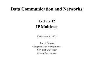
two senders, two receivers one router, infinite buffers no retransmission large delays when congested maximum achievable throughput lout lin : original data unlimited shared output link buffers Host A Host B Causes/costs of congestion: scenario 1 Transport Layer
one router, finite buffers sender retransmission of lost packet Causes/costs of congestion: scenario 2 Host A lout lin : original data l'in : original data, plus retransmitted data Host B finite shared output link buffers Transport Layer
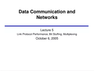
always: (goodput) “perfect” retransmission only when loss: retransmission of delayed (not lost) packet makes larger (than perfect case) for same l l l > = l l l R/2 in in in R/2 R/2 out out out R/3 lout lout lout R/4 R/2 R/2 R/2 lin lin lin a. b. c. Causes/costs of congestion: scenario 2 “costs” of congestion: • more work (retrans) for given “goodput” • unneeded retransmissions: link carries multiple copies of pkt Transport Layer
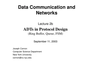
four senders multihop paths timeout/retransmit l l in in Host A Host B Causes/costs of congestion: scenario 3 Q:what happens as and increase ? lout lin : original data l'in : original data, plus retransmitted data finite shared output link buffers Transport Layer
Host A Host B Causes/costs of congestion: scenario 3 lout Another “cost” of congestion: • when packet dropped, any “upstream transmission capacity used for that packet was wasted! Transport Layer
Practical Performance • Ideal assumes infinite buffers and no overhead • Buffers are finite • Overheads occur in exchanging congestion control messages Transport Layer
End-end congestion control: no explicit feedback from network congestion inferred from end-system observed loss, delay approach taken by TCP Network-assisted congestion control: routers provide feedback to end systems single bit indicating congestion (SNA, DECbit, TCP/IP ECN, ATM) explicit rate sender should send at Approaches towards congestion control Two broad approaches towards congestion control: Transport Layer
Mechanisms for Congestion Control Transport Layer
Backpressure • If node becomes congested it can slow down or halt flow of packets from other nodes • May mean that other nodes have to apply control on incoming packet rates • Propagates back to source • Can restrict to logical connections generating most traffic • Used in connection oriented that allow hop by hop congestion control (e.g. X.25) • Not used in ATM Transport Layer
Choke Packet • Control packet • Generated at congested node • Sent to source node • e.g. ICMP source quench • From router or destination • Source cuts back until no more source quench message • Sent for every discarded packet, or anticipated • Rather crude mechanism Transport Layer
Implicit Congestion Signaling • Transmission delay may increase with congestion • Packet may be discarded • Source can detect these as implicit indications of congestion • Useful on connectionless (datagram) networks, e.g. IP based • Used in frame relay LAPF Transport Layer
Explicit Congestion Signaling • Network alerts end systems of increasing congestion • End systems take steps to reduce offered load • Backwards • Congestion avoidance in opposite direction to packet required • Forwards • Congestion avoidance in same direction as packet required • Used in ATM by ABR Service Transport Layer
Traffic Shaping • Smooth out traffic flow and reduce cell clumping • Token bucket Transport Layer
Token Bucket for Traffic Shaping Transport Layer
ABR: available bit rate: “elastic service” if sender’s path “underloaded”: sender should use available bandwidth if sender’s path congested: sender throttled to minimum guaranteed rate RM (resource management) cells: sent by sender, interspersed with data cells bits in RM cell set by switches (“network-assisted”) NI bit: no increase in rate (mild congestion) CI bit: congestion indication RM cells returned to sender by receiver, with bits intact Case study: ATM ABR congestion control Transport Layer
two-byte ER (explicit rate) field in RM cell congested switch may lower ER value in cell sender’ send rate thus minimum supportable rate on path EFCI bit in data cells: set to 1 in congested switch if data cell preceding RM cell has EFCI set, sender sets CI bit in returned RM cell Case study: ATM ABR congestion control Transport Layer
end-end control (no network assistance) sender limits transmission: LastByteSent-LastByteAcked CongWin Roughly, CongWin is dynamic, function of perceived network congestion How does sender perceive congestion? loss event = timeout or 3 duplicate acks TCP sender reduces rate (CongWin) after loss event three mechanisms: AIMD slow start conservative after timeout events CongWin rate = Bytes/sec RTT TCP Congestion Control Transport Layer
multiplicative decrease: cut CongWin in half after loss event TCP AIMD additive increase: increase CongWin by 1 MSS every RTT in the absence of loss events: probing Long-lived TCP connection Transport Layer
When connection begins, CongWin = 1 MSS Example: MSS = 500 bytes & RTT = 200 msec initial rate = 20 kbps available bandwidth may be >> MSS/RTT desirable to quickly ramp up to respectable rate TCP Slow Start • When connection begins, increase rate exponentially fast until first loss event Transport Layer
When connection begins, increase rate exponentially until first loss event: double CongWin every RTT done by incrementing CongWin for every ACK received Summary: initial rate is slow but ramps up exponentially fast time TCP Slow Start (more) Host A Host B one segment RTT two segments four segments Transport Layer
After 3 dup ACKs: CongWin is cut in half window then grows linearly But after timeout event: CongWin instead set to 1 MSS; window then grows exponentially to a threshold, then grows linearly Refinement Philosophy: • 3 dup ACKs indicates network capable of delivering some segments • timeout before 3 dup ACKs is “more alarming” Transport Layer
Q: When should the exponential increase switch to linear? A: When CongWin gets to 1/2 of its value before timeout. Implementation: Variable Threshold At loss event, Threshold is set to 1/2 of CongWin just before loss event Refinement (more) Transport Layer
Summary: TCP Congestion Control • When CongWin is below Threshold, sender in slow-start phase, window grows exponentially. • When CongWin is above Threshold, sender is in congestion-avoidance phase, window grows linearly. • When a triple duplicate ACK occurs, Threshold set to CongWin/2 and CongWin set to Threshold. • When timeout occurs, Threshold set to CongWin/2 and CongWin is set to 1 MSS. Transport Layer
TCP sender congestion control Transport Layer
TCP throughput • What’s the average throughout ot TCP as a function of window size and RTT? • Ignore slow start • Let W be the window size when loss occurs. • When window is W, throughput is W/RTT • Just after loss, window drops to W/2, throughput to W/2RTT. • Average throughout: .75 W/RTT Transport Layer
TCP Futures • Example: 1500 byte segments, 100ms RTT, want 10 Gbps throughput • Requires window size W = 83,333 in-flight segments • Throughput in terms of loss rate: • ➜ L = 2·10-10 Wow • New versions of TCP for high-speed needed! Transport Layer
Fairness goal: if K TCP sessions share same bottleneck link of bandwidth R, each should have average rate of R/K TCP connection 1 bottleneck router capacity R TCP connection 2 TCP Fairness Transport Layer
Two competing sessions: Additive increase gives slope of 1, as throughout increases multiplicative decrease decreases throughput proportionally Why is TCP fair? equal bandwidth share R loss: decrease window by factor of 2 congestion avoidance: additive increase Connection 2 throughput loss: decrease window by factor of 2 congestion avoidance: additive increase Connection 1 throughput R Transport Layer
Fairness and UDP Multimedia apps often do not use TCP do not want rate throttled by congestion control Instead use UDP: pump audio/video at constant rate, tolerate packet loss Research area: TCP friendly Fairness and parallel TCP connections nothing prevents app from opening parallel cnctions between 2 hosts. Web browsers do this Example: link of rate R supporting 9 cnctions; new app asks for 1 TCP, gets rate R/10 new app asks for 11 TCPs, gets R/2 ! Fairness (more) Transport Layer
Q:How long does it take to receive an object from a Web server after sending a request? Ignoring congestion, delay is influenced by: TCP connection establishment data transmission delay slow start Notation, assumptions: Assume one link between client and server of rate R S: MSS (bits) O: object size (bits) no retransmissions (no loss, no corruption) Window size: First assume: fixed congestion window, W segments Then dynamic window, modeling slow start Delay modeling Transport Layer
First case: WS/R > RTT + S/R: ACK for first segment in window returns before window’s worth of data sent Fixed congestion window (1) delay = 2RTT + O/R Transport Layer
Second case: WS/R < RTT + S/R: wait for ACK after sending window’s worth of data sent Fixed congestion window (2) delay = 2RTT + O/R + (K-1)[S/R + RTT - WS/R] Transport Layer
TCP Delay Modeling: Slow Start (1) Now suppose window grows according to slow start Will show that the delay for one object is: where P is the number of times TCP idles at server: - where Q is the number of times the server idles if the object were of infinite size. - and K is the number of windows that cover the object. Transport Layer
TCP Delay Modeling: Slow Start (2) • Delay components: • 2 RTT for connection estab and request • O/R to transmit object • time server idles due to slow start • Server idles: P =min{K-1,Q} times • Example: • O/S = 15 segments • K = 4 windows • Q = 2 • P = min{K-1,Q} = 2 • Server idles P=2 times Transport Layer
TCP Delay Modeling (3) Transport Layer
TCP Delay Modeling (4) Recall K = number of windows that cover object How do we calculate K ? Calculation of Q, number of idles for infinite-size object, is similar (see HW). Transport Layer