Download
1 / 20
210 likes | 241 Views
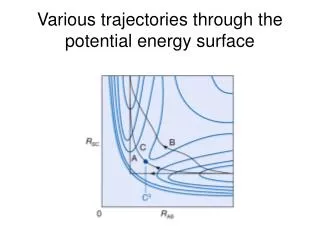
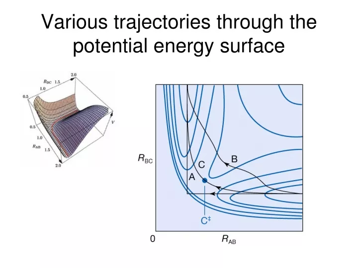
Various trajectories through the potential energy surface. Classical trajectories. The complex mode process: the activated complex survives for an extended period. Direct mode process:. 24.8(d) Quantum mechanical scattering theory.

E N D
Classical trajectories The complex mode process: the activated complex survives for an extended period. • Direct mode process:
24.8(d) Quantum mechanical scattering theory • Classic trajectory calculations do not recognize the fact that the motion of atoms, electrons, and nuclei is governed by quantum mechanics. • Using wave function to represent initially the reactants and finally products. • Need to take into account all the allowed electronic, vibrational, and rotational states populated by each atom and molecules in the system at a given temperature. • Use “channel” to express a group of molecules in well-defined quantum mechanically allowed state. • Many channels can lead to the desired product, which complicate the quantum mechanical calculations. • The cumulative reaction probability, N(E), the summation of all possible transitions that leads to products.
24.9 The investigation of reaction dynamics with ultrafast laser technique • Spectroscopic observation of the activated complex. pico: 10-12; femto: 10-15 activated complex often survive a few picoseconds. • Femtosecond spectroscopy (two pulses): • Controlling chemical reactions with lasers. mode-selective chemistry:using laser to excite the reactants to different vibrational states: Example: H + HOD reaction. Limitation: energy can be deposited and remains localized. combination of ultrafast lasers: Overall, it requires more sophisticated knowledge of how stimulation works.
24.10 The rate of electron transfer processes in homogeneous systems Consider electron transfer from a donor D to an acceptor A in solution D + A → D+ + A- v = kobs [D][A] Assuming that D, A and DA (the complex being formed first) are in equilibrium: D + A ↔ DA KDA = [DA]/([D][A]) = ka/ka’ Next, electron transfer occurs within the DA complex DA → D+A- vet = ket[DA] D+A- has two fates: D+A- → DA vr = kr[D+A- ] D+A- → D+ + A-vd = kd[D+A- ]
Electron transfer process • For the case kd>> kr: • When ket <<ka’: kobs≈ (ka/ka’)ket • Using transition state theory:
24.11 Theory of electron transfer processes • Electrons are transferred by tunneling through a potential energy barrier. Electron tunneling affects the magnitude of kv • The complex DA and the solvent molecules surrounding it undergo structural rearrangements prior to electron transfer. The energy associated with these rearrangements and the standard reaction Gibbs energy determine Δ±G (the Gibbs energy of activation).
24.11(a) Electron tunneling • An electron migrates from one energy surface, representing the dependence of the energy of DA on its geometry, to another representing the energy of D+A-. (so fast that they can be regarded as taking place in s stationary nuclear framework) • The factor kv is a measure of the probability that the system will convert from DA to D+A- at the intersection by thermal fluctuation.
Initially, the electron to be transferred occupies the HOMO of D • Nuclei rearrangement leads to the HOMO of DA and the LUMO of D+A- degenerate and electron transfer becomes energetically feasible.
24.12 Experimental results of electron transfer processes where λ is the reorganization energy
Decrease of electron transfer rate with increasing reaction Gibbs energy
Marcus cross-relation • *D + D+→ *D+ + D kDD • *A- + A → *A + A- kAA • Kobs = (kDD kAA K)1/2 Examples: Estimate kobs for the reduction by cytochrome c of plastocyanin, a protein containing a copper ion that shuttles between the +2 and +1 oxidation states and for which kAA = 6.6 x 10² M-1s-1 and E0 = 0.350 V.
Chapter 25Electron transfer in heterogeneous systems(Processes at electrodes)
Impacts on our society • Most of the modern method of generating electricity are inefficient, and the development of fuel cells could revolutionize the production and deployment of energy. • The inefficiency can be improved by knowing more about the kinetics of electrochemical processes. • Applications in organic and inorganic electrosynthesis. • Waste treatments.
25.8The electrode-solution interface • Electrical double layer Helmholtz layer model
Gouy-Chapman Model • This model explains why measurements of the dynamics of electrode processes are almost always done using a large excess of supporting electrolyte.
The Stern model of the electrode-solution interface • The Helmholtz model overemphasizes the rigidity of the local solution. • The Gouy-Chapman model underemphasizes the rigidity of local solution. • The improved version is the Stern model.
Outer potential • Inner potential • Surface potential • The potential difference between the points in the bulk metal (i.e. electrode) and the bulk solution is the Galvani potential difference which is the electrode potential discussed in chapter 7. The electric potential at the interface
The origin of the distance-independence of the outer potential
The connection between the Galvani potential difference and the electrode potential • Electrochemical potential (û) û = u + zFø • Discussions through half-reactions