Download
1 / 26
270 likes | 571 Views
Ultraviolet Light Process Model Evaluation. Presented by: Jennifer Hartfelder, P.E. Brown and Caldwell. Models to Evaluate UV Performance. USEPA Mathematical Protocol – USEPA Design Manual Municipal Wastewater Disinfection

E N D
Ultraviolet Light Process Model Evaluation Presented by: Jennifer Hartfelder, P.E. Brown and Caldwell
Models to Evaluate UV Performance • USEPA Mathematical Protocol – USEPA Design Manual Municipal Wastewater Disinfection • UVDIS – Software Developed by HydroQual, Inc. based on the USEPA Mathematical Protocol • NWRI/AWWARF Protocol – Ultraviolet Disinfection Guidelines for Drinking Water and Water Reuse
UV Process Design Model • Chick’s Law: N = Noe-kIt • N = bacterial concentration remaining after exposure to UV • No = initial bacterial concentration • k = rate constant • I = intensity of UV • t = time of exposure
USEPA - Step 2Calculate Intensity • Biological Assay • Direct Calculation Method
Average Intensity • Iavg = (nominal Iavg)(Fp)(Ft) • Fp = the ratio of the actual output of the lamps to the nominal output of the lamps • Ft = the ratio of the actual transmittance of the quartz sleeve or Teflon tubes to the nominal transmittance of the enclosure
USEPA - Step 3Determine Inactivation Rates • K = aIavgb
USEPA - Step 4Determine Dispersion Coefficient • Establish relationship between x and u • hL = cf(x)(u)2 • Plot log(u) and log(x) versus log(ux) • Dispersion number, d • d = E/(ux) • d = 0.03 to 0.05 • E = 50 to 200 cm2/sec
USEPA - Step 5Determine UV Loading • Plot log(N’/No) vs. Q/Wn and u vs. Q/Wn
USEPA - Step 6Establish Performance Goals • Np = cSSm • N’ = N - Np
USEPA - Step 7Calculate Reactor Sizing • Number of lamps required: • Q/Wn – determined from the log (N’/No) vs. maximum loading graphs developed in Step 5 for the N’ developed in Step 6 • Lamps required = Q/(Q/Wn)/Wn
Arc length Centerline spacing Watts output Quartz Sleeve Diameter No. of banks in series Aging Factor Fouling Factor Flow Dispersion Coefficient Average Intensity Number of lamps Staggered Percent transmissivity UVDIS Input
NWRI/AWWARF Protocol • Determine UV inactivation of selected microorganisms under controlled batch conditions by conducting a bioassay • Dose-Response Curves • Microorganism • MS-2 bacteriophage • E. coli • Pilot vs. full scale study
UV Dose • German drinking water standard: 40 mW-sec/cm2 • US wastewater industry standard: 30 mW-sec/cm2 • CDPHE WWTP design criteria: 30 mW-sec/cm2 • US reuse standard: 50 - 100 mW-sec/cm2 • NWRI/AWWARF based on upstream filtration: • Media - 100 mW-sec/cm2 • Membrane - 80 mW-sec/cm2 • Reverse Osmosis - 40 mW-sec/cm2
Protocol Evaluation • For peak hour conditions: • Q = 3.5 MGD (9,200 lpm) • SS = 45 mg/L • No = 1.50E+06 No./100 mL • N = 6,000 No./100 mL • Transmittance = 60% • Allowable headloss = 1.5 inches
Pros Apply same calculations to all systems Can be used for uniform, staggered, concentric, and tubular lamp arrays Cons Least conservative Assumes flow perpendicular to lamp USEPA Mathematical Protocol
Pros HydroQual is in the process of updating the program to address some of the cons More conservative than USEPA protocol Cons Less conservative than bioassay For low-pressure systems only For flow parallel to lamps only Dispersion coefficient, E, is assumed UVDIS
Pros Most conservative May assume a conservative required dose (50 to 100 mW-sec/cm2) Cons Bioassay tests have not been conducted yet for all systems Bioassay is costly Scale-up issues Bioassays have not used the same protocol (i.e., microorganism) More research on how to select required dose is necessary NWRI/AWWARF Protocol
Conclusions • Bioassay is most conservative sizing method • More research required: • Dose selection protective of human health • Scale-up issues • Target organism • Engineer should require a field performance test and performance bond