Download
1 / 39
390 likes | 513 Views
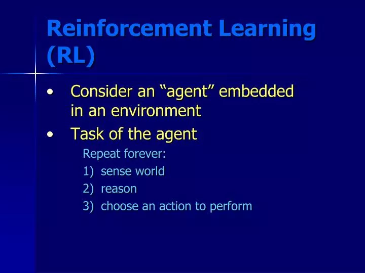
Reinforcement Learning (RL). Consider an “agent” embedded in an environment Task of the agent Repeat forever: sense world reason choose an action to perform. Definition of RL. Assume the world (ie, environment) periodically provides rewards or punishments (“reinforcements”)

E N D
Reinforcement Learning (RL) • Consider an “agent” embedded in an environment • Task of the agent Repeat forever: • sense world • reason • choose an action to perform
Definition of RL • Assume the world (ie, environment) periodically provides rewards or punishments (“reinforcements”) • Based on reinforcements received, learn how to better choose actions
Sequential Decision Problems Courtesy of A.G. Barto, April 2000 • Decisions are made in stages • The outcome of each decision is not fully predictable but can be observed before the next decision is made • The objective is to maximize a numerical measure of total reward (or equivalently, to minimize a measure of total cost) • Decisions cannot be viewed in isolation: need to balance desire for immediate reward with possibility of high future reward
Reinforcement Learning vs Supervised Learning • How would we use SL to train an agent in an environment? • Show action to choose in sample of world states – “I/O pairs” • RL requires much less of teacher • Must set up “reward structure” • Learner “works out the details” – i.e. writes a program to maximize rewards received
Embedded Learning Systems: Formalization • SE = the set of states of the world • e.g., an N-dimensional vector • “sensors” • AE = the set of possible actions an agent can perform • “effectors” • W = the world • R = the immediate reward structure W and R are the environment, can be probabilistic functions
Embedded learning Systems (formalization) W: SE x AE SE The world maps a state and an action and produces a new state R: SE x AE “reals” Provides rewards (a number) as a function of state and action (as in textbook). Can equivalently formalize as a function of state (next state) alone.
A Graphical View of RL • Note that both the world and the agent can be probabilistic, so W and R could produce probability distributions. • For now, assume deterministic problems The real world, W R, reward (a scalar) - indirect teacher an action sensory info The Agent
Common Confusion State need not be solely the current sensor readings • Markov Assumption Value of state is independent of path taken to reach that state • Can have memory of the past Can always create Markovian task by remembering entire past history
Need for Memory: Simple Example “out of sight, but not out of mind” T=1 learning agent opponent W A L L opponent T=2 learning agent W A L L Seems reasonable to remember opponent recently seen
State vs. Current Sensor Readings Rememberstate is what is in one’s head (past memories, etc) not ONLY what one currently sees/hears/smells/etc
Policies The agent needs to learn a policy E : SE AE Given a world state, SE, which action, AE, should be chosen? The policy, E, function Remember: The agent’s task is to maximize the total reward received during its lifetime
Policies (cont.) To construct E, we will assign a utility(U)(a number) to each state. • - is a positive constant < 1 • R(s, E, t) is the reward received at time t, assuming the agent follows policy E and starts in state s at t=0 • Note: future rewards are discounted by t-1
immediate reward received for going to state W(s,a) Future reward from further actions (discounted due to 1-step delay) The Action-Value Function We want to choose the “best” action in the current state So, pick the one that leads to the best next state (and include any immediate reward) Let
The Action-Value Function (cont.) If we can accurately learn Q (the action-value function), choosing actions is easy Choose a, where
U’s “stored” on states Q’s “stored” on arcs Qvs. UVisually action state state U(2) Key Q(1,i) states U(5) actions U(1) Q(1,ii) U(3) U(6) Q(1,iii) U(4)
Q-Learning (Watkins PhD, 1989) Let Qtbe our current estimate of the correct Q Our current policy is suchthat Our current utility-function estimate is - hence, the U table is embedded in the Q table and we don’t need to store both
Q-Learning (cont.) Determine actual reward and compare to predicted reward Adjust prediction to reduce error (1 ) I.e., follow the current policy Assume we are in state St “Run the program”(1) for awhile (n steps)
How Many Actions Should We Take Before Updating Q? Why not do so after each action? • “1 – Step Q learning” • Most common approach
Exploration vs. Exploitation In order to learn about better alternatives, we can’t always follow the current policy (“exploitation”) Sometimes, need to try “random” moves (“exploration”)
Exploration vs. Exploitation (cont) Approaches 1) p percent of the time, make a random move; could let 2) Prob(picking action A in state S) Exponentia-ting gets rid of negative values
One-Step Q-Learning Algo 0. S initial state 1. If random # P then a = random choice Else a = t(S) 2. Snew W(S, a) Rimmed R(Snew) • Q(S, a) Rimmed + g maxa’ Q(Snew, a’) 4. S Snew • Go to 1 Act on world and get reward
In Stochastic World, Don’t Trash Current Q Entirely… Change Line 3: • Q(S, a) Rimmed + g maxa’ Q(Snew, a’) To: Q(S, a) α [Rimmed + g maxa’ Q(Snew, a’)] + (1-α) Q(S, a)
A Simple Example (of Q-learning - with updates after each step, ie N =1) S1 R = 1 Let = 2/3 Q = 0 S0 R = 0 Q = 0 Q = 0 Q = 0 S3 R = 0 Algo: Pick State +Action S2 R = -1 Q = 0 S4 R = 3 Q = 0 Repeat (deterministic world, so α=1)
A Simple Example (Step 1)S0 S2 S1 R = 1 Let = 2/3 Q = 0 S0 R = 0 Q = 0 Q = 0 Q = -1 S3 R = 0 Algo: Pick State +Action S2 R = -1 Q = 0 S4 R = 3 Q = 0 Repeat (deterministic world, so α=1)
A Simple Example (Step 2)S2 S4 S1 R = 1 Let = 2/3 Q = 0 S0 R = 0 Q = 0 Q = 0 Q = -1 S3 R = 0 Algo: Pick State +Action S2 R = -1 Q = 0 S4 R = 3 Q = 3 Repeat (deterministic world, so α=1)
A Simple Example (Step ) S1 R = 1 Let = 2/3 Q = 1 S0 R = 0 Q = 0 Q = 0 Q = 1 S3 R = 0 Algo: Pick State +Action S2 R = -1 Q = 0 S4 R = 3 Q = 3 Repeat (deterministic world, so α=1)
Q-Learning: Implementation Details Remember, conceptually we are filling in a huge table States S0 S1 S2 . . . Sn Actions . . . a b c . . . z Tables are a very verbose representationof a function . . . Q(S2, c)
Q-Learning: Convergence Proof • Applies to Q tables and deterministic, Markovian worlds. Initialize Q’s 0 or random finite. • Theorem: if every state-action pair visited infinitely often, 0≤<1, and |rewards| ≤ C (some constant), then s, a the approx. Q table (Q) the true Q table (Q) ^
Q-Learning Convergence Proof (cont.) • Consider the max error in the approx. Q-table at step t: • The max is finite since |r| ≤ C, so max || +C+Cγ • Since finite, we have finite, i.e. initial max error is finite
Q-Learning Convergence Proof (cont.) Let s’ be the state that results from doing action a in state s. Consider what happens when we visit s and do a at step t + 1: Next state Current state By def’n of Q (notice best a in s’ might be different) By Q-learning rule (one step)
Q-Learning Convergence Proof (cont.) ^ = | maxa’ Qt(s’, a’) – maxa’’ Q(s’, a’’) | By algebra ^ ≤ maxa’’’ | Qt(s’, a’’’) – Q(s’, a’’’) | Since max of all differences is as big as a particular one ^ ≤ maxs’’,a’’’ | Qt(s’’, a’’’) – Q(s’’, a’’’) | Max at s’ ≤ max at any s = Δt Plugging in defn of Δt
Q-Learning Convergence Proof (cont.) • Hence, every time, after t, we visit an <s, a>, its Q value differs from the correct answer by no more than Δt • Let To=to (i.e. the start) and TN be the first time since TN-1 where every<s, a> visited at least once • Call the time between TN-1 and TN, a complete interval ClearlyΔTN≤ ΔTN-1
Q-Learning Convergence Proof (concluded) • That is, every complete interval, Δt is reduced by at least • Since we assumed every <s, a> pair visited infinitely often, we will have an infinite number of complete intervals Hence, lim Δt = 0 t
Q (S, a) Q (S, b) . . . . . Q (S, z) Representing Q Functions More Compactly We can use some other function representation(eg, neural net) to compactly encode this big table Second argument is a constant An encoding of the state (S) Each input unit encodes a property of the state (eg, a sensor value) Or could have one net for each possible action
Q Tables vs Q Nets Given: 100 Boolean-valued features 10 possible actions Size of Q table 10 * 2 to the power of 100 Size of Q net (100 HU’s) 100 * 100 + 100 * 10 = 11,000 # of possible states Weights between inputs and HU’s Weights between HU’s and outputs
Why Use a Compact Q-Function? • Full Q table may not fit in memory for realistic problems • Can generalize across states, thereby speeding up convergence i.e., one example “fills” many cells in the Q table
SARSA vs. Q-Learning (1994, 1996) (1989) Exploring can be hazardous! Should we learn to consider its impact? The Cliff-Walking Task(pg 150 of Sutton + Barto RL Text) Safe route R=-1 for all of these R=0 Optimal path -if no exploration! What would Q-Learning learn?
SARSA uses actual next action (still chosen via explore-exploit strategy, e.g. soft-max or “coin-flip”) actual - SARSA also converges a’ a’’ a’ s Notice that in Q learning, (currently) non-optimal moves do not impact the Q function best s’ R SARSA = State Action Reward State Action SARSA Standard Q-Learning Q(s,a) Q(s,a) + [ R + Q(s’, a’) – Q(s,a) ] Q(s,a) Q(s,a) + [ R + max Q(s’, a’’) – Q(s,a) ]
Sample Results:Cliff-Walking Task optimal SARSA Total Reward Until Goal Q-Learning Episodes (ie from Start to Goal) (prob of random move = 0.1) SARSA learns to avoid ‘pitfalls’ while in exploration phase (always need to explore if in a real-world situation?)