Download
1 / 31
310 likes | 445 Views
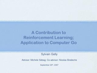
Chapter 3: The Reinforcement Learning Problem. describe the RL problem we will be studying for the remainder of the course present idealized form of the RL problem for which we have precise theoretical results;

E N D
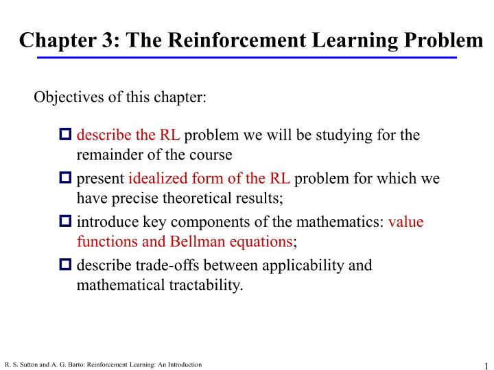
Chapter 3: The Reinforcement Learning Problem • describe the RL problem we will be studying for the remainder of the course • present idealized form of the RL problem for which we have precise theoretical results; • introduce key components of the mathematics: value functions and Bellman equations; • describe trade-offs between applicability and mathematical tractability. Objectives of this chapter: R. S. Sutton and A. G. Barto: Reinforcement Learning: An Introduction
r r r . . . . . . t +1 t +2 s s t +3 s s t +1 t +2 t +3 a a a a t t +1 t +2 t t +3 The Agent-Environment Interface R. S. Sutton and A. G. Barto: Reinforcement Learning: An Introduction
The Agent Learns a Policy • Reinforcement learning methods specify how the agent changes its policy as a result of experience. • Roughly, the agent’s goal is to get as much reward as it can over the long run. R. S. Sutton and A. G. Barto: Reinforcement Learning: An Introduction
Getting the Degree of Abstraction Right • Time steps need not refer to fixed intervals of real time. • Actions can be low level (e.g., voltages to motors), or high level (e.g., accept a job offer), “mental” (e.g., shift in focus of attention), etc. • States can low-level “sensations”, or they can be abstract, symbolic, based on memory, or subjective (e.g., the state of being “surprised” or “lost”). • An RL agent is not like a whole animal or robot, which consist of many RL agents as well as other components. • The environment is not necessarily unknown to the agent, only incompletely controllable. • Reward computation is in the agent’s environment because the agent cannot change it arbitrarily. R. S. Sutton and A. G. Barto: Reinforcement Learning: An Introduction
Goals and Rewards • Is a scalar reward signal an adequate notion of a goal?—maybe not, but it is surprisingly flexible. • A goal should specify what we want to achieve, not how we want to achieve it. • A goal must be outside the agent’s direct control—thus outside the agent. • The agent must be able to measure success: • explicitly; • frequently during its lifespan. R. S. Sutton and A. G. Barto: Reinforcement Learning: An Introduction
Returns Episodic tasks: interaction breaks naturally into episodes, e.g., plays of a game, trips through a maze. where T is a final time step at which a terminal stateis reached, ending an episode. R. S. Sutton and A. G. Barto: Reinforcement Learning: An Introduction
Returns for Continuing Tasks Continuing tasks: interaction does not have natural episodes. Discounted return: R. S. Sutton and A. G. Barto: Reinforcement Learning: An Introduction
An Example Avoidfailure: the pole falling beyond a critical angle or the cart hitting end of track. As anepisodic task where episode ends upon failure: As acontinuingtaskwith discounted return: In either case, return is maximized by avoiding failure for as long as possible. R. S. Sutton and A. G. Barto: Reinforcement Learning: An Introduction
Another Example Get to the top of the hill as quickly as possible. Return is maximized by minimizing number of steps reach the top of the hill. R. S. Sutton and A. G. Barto: Reinforcement Learning: An Introduction
A Unified Notation • In episodic tasks, we number the time steps of each episode starting from zero. • We usually do not have to distinguish between episodes, so we write instead of for the state at step t of episode j. • Think of each episode as ending in an absorbing state that always produces reward of zero: • We can cover all cases by writing R. S. Sutton and A. G. Barto: Reinforcement Learning: An Introduction
The Markov Property • By “the state” at step t, the book means whatever information is available to the agent at step t about its environment. • The state can include immediate “sensations,” highly processed sensations, and structures built up over time from sequences of sensations. • Ideally, a state should summarize past sensations so as to retain all “essential” information, i.e., it should have the Markov Property: R. S. Sutton and A. G. Barto: Reinforcement Learning: An Introduction
Markov Decision Processes • If a reinforcement learning task has the Markov Property, it is basically a Markov Decision Process (MDP). • If state and action sets are finite, it is a finite MDP. • To define a finite MDP, you need to give: • state and action sets • one-step “dynamics” defined by transition probabilities: • reward probabilities: R. S. Sutton and A. G. Barto: Reinforcement Learning: An Introduction
An Example Finite MDP • At each step, robot has to decide whether it should (1) actively search for a can, (2) wait for someone to bring it a can, or (3) go to home base and recharge. • Searching is better but runs down the battery; if runs out of power while searching, has to be rescued (which is bad). • Decisions made on basis of current energy level: high, low. • Reward = number of cans collected Recycling Robot R. S. Sutton and A. G. Barto: Reinforcement Learning: An Introduction
Recycling Robot MDP R. S. Sutton and A. G. Barto: Reinforcement Learning: An Introduction
Value Functions • The value of a state is the expected return starting from that state; depends on the agent’s policy: • The value of taking an action in a stateunder policy p is the expected return starting from that state, taking that action, and thereafter following p : R. S. Sutton and A. G. Barto: Reinforcement Learning: An Introduction
Bellman Equation for a Policy p The basic idea: So: Or, without the expectation operator (Bellman equation for Vp): R. S. Sutton and A. G. Barto: Reinforcement Learning: An Introduction
More on the Bellman Equation This is a set of equations (in fact, linear), one for each state. The value function for p is its unique solution. Backup diagrams: R. S. Sutton and A. G. Barto: Reinforcement Learning: An Introduction
Grid world • Actions: north, south, east, west; deterministic. • If would take agent off the grid: no move but reward = –1 • Other actions produce reward = 0, except actions that move agent out of special states A (+10) and B (+5) to their goals as shown. State-value function for equiprobable random policy; g = 0.9 Note that learning the policy that maximizes the award is an objective of RL R. S. Sutton and A. G. Barto: Reinforcement Learning: An Introduction
Grid world % Example 3.8 % matrix is scanned column wise % action - going north clear all; R=zeros(4,25); % next states S_prime(1,1)=1; S_prime(1,2:25)=(1:24); S_prime(1,11)=11; S_prime(1,21)=21; % reward in north direction for i=0:4 R(1,i*5+1)=-1; end; % action - going east S_prime(2,1:20)=(6:25); S_prime(2,21:25)=(21:25); % reward in east direction R(2,21:25)=-1; % action - going south S_prime(3,1:24)=(2:25); S_prime(3,5:5:25)=(5:5:25); % reward in south direction R(3,5:5:25)=-1; % action - going west S_prime(4,6:25)=(1:20); S_prime(4,1:5)=(1:5); % reward in west direction R(4,1:5)=-1; % special states for i=1:4 S_prime(i,6)=10; S_prime(i,16)=18; R(i,6)=10; R(i,16)=5; end; R. S. Sutton and A. G. Barto: Reinforcement Learning: An Introduction
Grid world Vpi=reshape(Vpi,5,5) % Vpi = % 3.3253 8.8065 4.4398 5.3320 1.4968 % 1.5362 3.0064 2.2612 1.9157 0.5529 % 0.0652 0.7517 0.6852 0.3681 -0.3946 % -0.9582 -0.4202 -0.3407 -0.5720 -1.1703 % -1.8410 -1.3287 -1.2127 -1.4068 -1.9593 % initialize variables Veps=0.01; delV=1; gamma=0.9; Vpi=zeros(1,25); % iterate until convergence while delV>Veps % Bellman equation Vpi_new=0.25*sum(R+gamma*Vpi(S_prime)); delV=norm(Vpi_new-Vpi); Vpi=Vpi_new; end; 0.25 R combines this product R. S. Sutton and A. G. Barto: Reinforcement Learning: An Introduction
% direct solution can be obtained in a linear system T=eye(25); for i=1:25 for j=1:4 T(i,S_prime(j,i)')=T(i,S_prime(j,i)')-0.25*gamma; end; end; Vpi=inv(T)*0.25*sum(R)'; Diagonal matrix for Vp(s), and effect of Vp(s’) Rewards on the rhs More on the Bellman Equation Since this is a set of linear equations, they can be solved without iterations (and exactly) by direct inverse. Vpi=reshape(Vpi,5,5) % Vpi = % 3.3090 8.7893 4.4276 5.3224 1.4922 % 1.5216 2.9923 2.2501 1.9076 0.5474 % 0.0508 0.7382 0.6731 0.3582 -0.4031 % -0.9736 -0.4355 -0.3549 -0.5856 -1.1831 % -1.8577 -1.3452 -1.2293 -1.4229 -1.9752 R. S. Sutton and A. G. Barto: Reinforcement Learning: An Introduction
Golf • State is ball location • Reward of –1 for each stroke until the ball is in the hole • Value of a state? • Actions: • putt (use putter) • driver (use driver) • puttsucceeds anywhere on the green R. S. Sutton and A. G. Barto: Reinforcement Learning: An Introduction
Optimal Value Functions • For finite MDPs, policies can be partially ordered: • There is always at least one (and possibly many) policies that is better than or equal to all the others. This is an optimal policy. We denote them all p *. • Optimal policies share the same optimal state-value function: • Optimal policies also share the same optimal action-value function: This is the expected return for taking action a in state s and thereafter following an optimal policy. R. S. Sutton and A. G. Barto: Reinforcement Learning: An Introduction
Optimal Value Function for Golf • We can hit the ball farther with driver than with putter, but with less accuracy • Q*(s,driver) gives the value or using driver first, then using whichever actions are best R. S. Sutton and A. G. Barto: Reinforcement Learning: An Introduction
Bellman Optimality Equation for V* The value of a state under an optimal policy must equal the expected return for the best action from that state: The relevant backup diagram: is the unique solution of this system of nonlinear equations. R. S. Sutton and A. G. Barto: Reinforcement Learning: An Introduction
Bellman Optimality Equation for Q* The relevant backup diagram: is the unique solution of this system of nonlinear equations. R. S. Sutton and A. G. Barto: Reinforcement Learning: An Introduction
Why Optimal State-Value Functions are Useful Any policy that is greedy with respect to is anoptimal policy. Therefore, given , one-step-ahead search produces the long-term optimal actions. E.g., back to the grid world: R. S. Sutton and A. G. Barto: Reinforcement Learning: An Introduction
What About Optimal Action-Value Functions? Given , the agent does not even have to do a one-step-ahead search: % find the optimum state value while delV>Veps [Vpi_new,I]=max(R+gamma*Vpi(S_prime)); delV=norm(Vpi_new-Vpi); Vpi=Vpi_new; end; % determine the optimum policy Reward=R+gamma*Vpi(S_prime); for i=1:25 Optimum_policy(:,i)=(Reward(:,i)==Reward(I(i),i)); end; norm=sum(Optimum_policy); for i=1:25 Optimum_policy(:,i)=Optimum_policy(:,i)./norm(i); end R. S. Sutton and A. G. Barto: Reinforcement Learning: An Introduction
What About Optimal Action-Value Functions? Vpi=reshape(Vpi,5,5) % Vpi = % 21.9694 24.4104 21.9694 19.4104 17.4694 % 19.7724 21.9694 19.7724 17.7952 16.0115 % 17.7952 19.7724 17.7952 16.0115 14.4104 % 16.0115 17.7952 16.0115 14.4104 12.9694 % 14.4104 16.0115 14.4104 12.9694 11.6724 Optimum_policy % First 14 columns of Optimum_policy = % Columns 1 through 7 % 0 0.5000 0.5000 0.5000 0.5000 0.2500 1.0000 % 1.0000 0.5000 0.5000 0.5000 0.5000 0.2500 0 % 0 0 0 0 0 0.2500 0 % 0 0 0 0 0 0.2500 0 % Columns 8 through 14 % 1.0000 1.0000 1.0000 0 0.5000 0.5000 0.5000 % 0 0 0 0 0 0 0 % 0 0 0 0 0 0 0 % 0 0 0 1.0000 0.5000 0.5000 0.5000 R. S. Sutton and A. G. Barto: Reinforcement Learning: An Introduction
Solving the Bellman Optimality Equation • Finding an optimal policy by solving the Bellman Optimality Equation requires the following: • accurate knowledge of environment dynamics; • we have enough space an time to do the computation; • the Markov Property. • How much space and time do we need? • polynomial in number of states (via dynamic programming methods; Chapter 4), • BUT, number of states is often huge (e.g., backgammon has about 10**20 states). • We usually have to settle for approximations. • Many RL methods can be understood as approximately solving the Bellman Optimality Equation. R. S. Sutton and A. G. Barto: Reinforcement Learning: An Introduction
Agent-environment interaction States Actions Rewards Policy: stochastic rule for selecting actions Return: the function of future rewards agent tries to maximize Episodic and continuing tasks Markov Property Markov Decision Process Transition probabilities Expected rewards Value functions State-value function for a policy Action-value function for a policy Optimal state-value function Optimal action-value function Optimal value functions Optimal policies Bellman Equations The need for approximation Summary R. S. Sutton and A. G. Barto: Reinforcement Learning: An Introduction