Download
1 / 38
380 likes | 414 Views
Data Compression. Outline Image Compression (GIF, JPEG) Video Compression (MPEG) Audio Compression (MP3). Why Compression?. Reduce bandwidth requirements (obvious) Reduce memory requirements (also obvious) Fundamental tradeoff between host processing and network bandwidth

E N D
Data Compression Outline Image Compression (GIF, JPEG) Video Compression (MPEG) Audio Compression (MP3) CMSC 332
Why Compression? • Reduce bandwidth requirements (obvious) • Reduce memory requirements (also obvious) • Fundamental tradeoff between host processing and network bandwidth • Depending on link speed, cost of processing (compression/decompression) may be more than offset by decrease in transfer time (though not always) CMSC 332
To Compress or Not To Compress • Bc = average bandwidth at which data can be pushed through compressor/decompressor in series • Bn = network bandwidth (including network processing) • r = compression ratio • x = number of uncompressed bytes to send • Assume: all data compressed before any transmitted • Cost to send uncompressed: x/Bn • Cost to send compressed: x/Bc + x/(rBn) • We win if: x/Bc + x/(rBn) < x/Bn • Equivalently: Bc > r/(r-1) × Bn CMSC 332
Coding and Compression • Before compressing, might as well encode data using fewest bits possible • Huffman Codes: if you know the relative probabilities with which symbols appear in data, you can use this to code more efficiently by assigning bits to symbols to minimize number of bits required • Ex. To encode letters of alphabet, need 5 bits. If letter R occurs 50% of time, however, then use fewer bits to encode R, more bits to encode letters like Z, X, etc. CMSC 332
Compression Overview • Lossless • data received = data sent • used for executables, text files, numeric data • Lossy • data received does not equal data sent • used for images, video, audio • Why do this? • We often don’t notice the difference since images, etc, can contain more information than humans can perceive (though radiologist, e.g., would want lossless images) • Better compression ratios (can be an order of magnitude better) CMSC 332
Run Length Encoding (RLE) • Replace consecutive occurrence of given symbol with symbol plus count of how many times it appears. • Example: AAABBCDDDD encoding as 3A2B1C4D • Can increase size for data with much variation (e.g., some images) since it takes two bytes to represent a non-repeated symbol • Can be used to compress digital images by comparing adjacent pixel values and encoding only the changes • Can achieve 8-to-1 compression ratio CMSC 332
Differential Pulse Code Modulation • (DPCM): Output a reference symbol and then for each succeeding symbol output difference between symbol and reference • Example AAABBCDDDD encoding as A0001123333 • Key benefit: when differences are small, they can be encoded with fewer bits than the symbols themselves • E.g. in above example, differences in range 0-3 can be encoded with 2 bits, while character takes 7 or 8. • change reference symbol if delta becomes too large • works better than RLE for many digital images (1.5-to-1) since small changes between pixels CMSC 332
Delta Encoding • Encode symbol as difference between previous one • Ex. AAABBCDDDD becomes A001011000 • Works well on images where adjacent pixel values are similar • Can perform RLE after delta encoding, since can be long strings of 0s CMSC 332
Dictionary-Based Methods • Build dictionary of common terms • variable length strings • Transmit index into dictionary for each term • Lempel-Ziv (LZ) is the best-known example (used by Unix compress() function) • Ex. Dictionary has 25,000 entries (words), the word “compression” is one of them. It takes 15 bits to index into dictionary, as opposed to 77 bits to encode compression in 7 bit ASCII CMSC 332
Dictionary-Based Methods • Commonly achieve 2-to-1 ratio on text • Problem: how to build the dictionary • Static • What if word isn’t there? • Must be tailored for data being compressed • Adaptive: must send the dictionary with the data in order to allow decoding. • Used by LZ • Extensive research on this problem CMSC 332
Using LZ to Compress GIF • First reduce 24-bit color to 8-bit color • Identify colors used in picture, pick 256 colors which most closely approximate colors in picture • Note this is lossy for pictures with more than 256 colors • Treat common sequence of pixels as terms in dictionary • Not uncommon to achieve 10-to-1 compression (x3) (though pictures of “natural scenes” typically do not achieve this ratio) CMSC 332
JPEG compression Source Compressed image image DCT Quantization Encoding Image Compression • JPEG: Joint Photographic Expert Group (ISO/ITU) • Lossy still-image compression • Three phase process • process in 8x8 pixel chunks (macroblock) • greyscale: each pixel is a single 8 bit value (for now) • DCT: transforms signal from spatial domain into an equivalent signal in the frequency domain (lossless) • apply a quantization to the results (lossy) • RLE-like encoding (lossless) CMSC 332
DCT Phase • Takes 8 8 pixel matrix as input and outputs 8 8 matrix of frequency coefficients • Spatial frequency intuition: Moving across a picture in x direction, pixel values change as function of x. • Large variation => low spacial frequency (gross detail) • Small variation => high spacial frequency (fine detail) • Idea: separate gross (essential) features from fine (perhaps imperceptible) features CMSC 332
DCT and Inverse DCT DCT(0,0) is called the DC coefficient, an average of the 64 input pixels. The rest are AC coefficients. CMSC 332
Quantization Phase • This is the lossy phase • Drop insignificant bits of frequency coefficients • Number of bits dropped is frequency dependent • Quantization equation: QuantizedValue(i,j)=IntegerRound(DCT(i,j)/Quantum(i,j)) IntegerRound(x) = CMSC 332
More Quantization • IntegerRound(x)is (not surprisingly) just rounding to the nearest integer • So, think about what quantization does: if range of potential starting values is 0-100, and quantum is 20, then by dividing and rounding, we effectively create 6 classes: • [0-10) gets mapped to 0 • [10-30) gets mapped to 1 • [30-50) gets mapped to 2 • [90-100] gets mapped to 5 CMSC 332
More Quantization • So now think about what happens when you try to get the original values back. Since we roughly found the classes by dividing by 20, to get original value back, we should multiply 20: • What was mapped to 0 gets changed back to 0 • What was mapped to 1 gets changed back to 20 • What was mapped to 2 gets changed back to 40 • So essentially everything in [0-10) becomes 0, everything in [10-30) becomes 20, and so on. CMSC 332
Still more Quantization • Now, if the quantum value was 50 rather than 20, then we would end up (by the same process) with 3 classes: • [0-25) which after quantization/reverse quant. becomes 0 • [25-75) which becomes 50 • [75-100] which becomes 100 • Bottom line: larger the quantum, the more information is lost in the quantization/reverse quantization process. This is the lossy part of JPEG CMSC 332
Quantization (cont.) • Quantization Table 3 5 7 9 11 13 15 17 5 7 9 11 13 15 17 19 7 9 11 13 15 17 19 21 9 11 13 15 17 19 21 23 11 13 15 17 19 21 23 25 13 15 17 19 21 23 25 27 15 17 19 21 23 25 27 29 17 19 21 23 25 27 29 31 • Decompression equation is: DCT(i,j) = QuantizedValue(i,j) × Quantum(i,j) • Ex. If DC coefficient is 25, then QuantizedValue(0,0) is 8. Coefficient would be restored as 24. CMSC 332
Encoding • Encoding done in order given below. • RLE used, followed by a Huffman code • Also, DC coefficients for macroblock are encoded using difference from DC coefficient of previous macroblock, since usually little change from block to block and DC coefficient contains much info. CMSC 332
Color • RGB: represent each pixel as three components, corresponding to red, green, and blue • YUV: also represent each pixel as three components • One luminance (Y) • Two chrominance (U and V) • Coordinates rotated to better correspond to human vision (which is not uniformly sensitive to colors) • We distinguish luminance much better than color CMSC 332
Color (cont.) • Images “overlaid” to produce picture, with each component processed as discussed above. • JPEG not limited to three components • Balancing compression versus fidelity • E.g. by changing quantization table • Rough compression ratio of 30:1 for 24 bit color • First reduce by factor of 3 down to 8 bits • Then by another factor of 10 using processing above CMSC 332
MPEG • Motion Picture Expert Group • Lossy compression of video • First approximation: JPEG on each frame, but must… • Also remove inter-frame redundancy • Extremely complicated, since it gives much encoding flexibility • We’ll focus here more on decoding side, since in many cases encoding is done offline. CMSC 332
Input Frame 1 Frame 2 Frame 3 Frame 4 Frame 5 Frame 6 Frame 7 stream MPEG compression Forward prediction Compressed I frame B frame B frame P frame B frame B frame I frame stream Bidirectional prediction MPEG (cont) • Frame types • I frames: intrapicture (reference frame; self-contained) • P frames: predicted picture (specifies difference from prev. I) • B frames: bidirectional predicted picture (interpolation of I,P) • Example sequence transmitted as I P B B I B B (?!) CMSC 332
MPEG (cont.) • I frames compressed similar to JPEG, but with 16×16 macroblock • Uses YUV scheme with U,V components down sampled to 8×8 (since humans less sensitive to color) CMSC 332
MPEG (cont.) • P, B frames also processed in macroblocks • Intuitively, these capture motion in frame • P frames: depend on one reference frame • B frames: • Usually depend on one or two reference frames • Can be encoded in same manner as I frame, if motion picture changing too rapidly • Each macroblock contains type field indicating which encoding it used CMSC 332
B Frame Bidirectional Predictive Encoding • B frame macroblock represented as a four-tuple • Coordinate for macroblock in frame • Motion vector relative to previous reference frame • Motion vector relative to subsequent reference frame • Delta () for each pixel in macroblock indicating how much pixel has changed relative to two reference pixels. • Where Fp, Ff represent past and future reference frames CMSC 332
B Predictive Encoding (cont.) • values encoded same as pixels in I frame • Run through DCT, then quantized • Since typically small, most DCT coefficients 0 after quantization, so they are effectively compressed • A problem: When encoding B or P frames, where do we put the macroblocks? • I.e. macroblock for B should match one for I, but not necessarily in same position (in fact, motion vectors specify the required direction) • Need to pick direction such that delta values as small as possible (called the motion estimation problem) • One reason why encoding takes longer than decoding CMSC 332
Performance • Typical compression ratio 90:1, sometimes as high as 150:1 • Values for I frames are 30:1 (since it’s really just JPEG—and assuming that 24 bit color reduced to 8 bit) • For P and B frames compression ratio is much smaller • Real-time MPEG encoding can be done in hardware—software is catching up • Decompression typically done in software (MPEG video boards do nothing more than color lookup) • Processors not fast enough to perform 30 frames/sec software decoding • 400MHz processor can run 20 frames/sec with 640×480stream CMSC 332
Transmitting MPEG • Groups of pictures (GOP) • SeqHdr: • size of each picture in GOP, measured in pixels and macroblocks • Interpicture prediod (in s) • Two quantization matrices (one for I frames, one for P and B frames) • Thus can change both quantization and frame rate at GOP granularity CMSC 332
Transmitting MPEG • GOPHdr followed by pictures in GOP • GOPHdr: • Number of pictures in GOP • Synchronization information for GOP (when GOP should play relative to beginning of video) • Picture: PictureHdr plus slices (regions, such as one horizontal line) • PictureHdr: • Type of picture (I,B, or P) • Picture specific quantization table CMSC 332
Transmitting MPEG • Slice: SliceHdr plus macroblocks • SliceHdr: • Vertical position of slice • Quantization table (well, just scaling factor) • Macroblocks: • MBHdr: block address within picture • Data for six blocks within the macroblock • 4 blocks of Y components • 1 each of U and V CMSC 332
Transmitting MPEG CMSC 332
TCP or UDP? • TCP nice since no need to packetize stream, but retransmission causes unacceptable latency with interactive video • UDP avoids retransmission, but packetizing is issue: • Want to break stream at points such that if packet is lost, it’s not a major problem (I.e. confine effects of lost packet to single macroblock) • Packet loss a problem since packets are differentiated (QoS here?) CMSC 332
More than just bandwidth… • Need to know application’s latency constraints • Combination of I,B, and P frames critical • Ex. I B B B B P B B B B I • Sender must delay four B frames until I or P that follows is available • At 15 frames/sec (frame per 67 ms), first B frame delayed 268ms plus network latency, much more than 100ms threshold for interactive video (based on human perception) CMSC 332
MP3 • MPEG standard for encoding audio from motion picture (MPEG also describes how to interleave audio, video streams) • A problem: • CD quality: sampled at 44.1 KHz (sample collected once every 23s). Samples are 16 bits, so stream is 1.41 Mbps • Telephone quality audio: 8 bit samples at sampling rate of 8KHz => 64Kbps stream (speed of ISDN link) CMSC 332
It’s much worse than this… • CD synchronization and error correcting requires that 49 bits be used to encode each 16 bit sample, so real bit rate is 4.32 Mbps. • MP3: Layer III level of MPEG encoding • Split audio stream into frequency bands • Break subbands into blocks similar to MPEG macroblocks (except these can vary from 64 to 1024 sampes, with sizes depending on distortion effects) • Use modified DCT, quantize, then Huffman encode CMSC 332
MP3 • Key is in how many subbands to use, and how many bits for each subband to produce highest quality audio for given target bit rate • Governed by psychoacoustic models (oooooh!) • MP3 dynamically changes quantization tables to achieve desired effect • After compression, subbands packeged into fixed-size frames • Hdr includes synchronization info, and info on number of bits used to encode each subband • Not a good idea to drop audio frames (we hear the difference) CMSC 332