Download
1 / 77
770 likes | 1.05k Views
LAMINAR PREMIXED FLAMES. Overview. Applications: Heating appliances Bunsen burners Burner for glass product manufacturing Importance of studying laminar premixed flames : Some burners use this type of flames as shown by examples above.

E N D
Overview Applications: • Heating appliances • Bunsen burners • Burner for glass product manufacturing Importance of studying laminar premixed flames: • Some burners use this type of flames as shown by examples above. • Prerequisite to the study of turbulent premixed flames. Both have the same physical processes and many turbulent flame theories are based on underlying laminar flame structure.
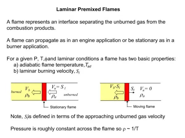
PHYSICAL DESCRIPTION Physical characteristics • Figure 1 shows typical flame temperature profile, mole fraction of reactants, R, and volumetric heat release, . • Velocity of reactants entering the flame, u = flame propagation velocity, SL • Products heated product density (b) < reactant density (u). Continuity requires that burned gas velicity, b >= unburned gas vel., u uSL A = uu A = bb A (1)
For a typical hydrocarbon-air flame at Patm, u/b 7 considerable acceleration of the gas flow across the flame (b tou). Fig. 1 Laminar flame structure, temperature and heat rate profiles based on experiments of Friedman and Burke
A flame consists of 2 zones: • Preheat zone, where little heat is released • Reaction zone, where the bulk of chemical energy is released Reaction zone consists of 2 regions: • Thin region(less than a millimeter), where reactions are very fast • Wide region (several millimeters), where reactions are slow
In thin region (fast reaction zone),destruction of the fuel molecules and creation of many intermediate species occur. This region is dominated by bimolecular reactions to produce CO. • Wide zone (slow reaction zone) is dominated by radical recombination reactions and final burnout of CO via CO + OH CO2 +H Flame colours in fast-reaction zone: • If air > stoichiometric proportions, excited CH radicals result in blue radiation. • If air < stoichiometric proportions, the zone appears blue-green as a result of radiation from excited C2.
In both flame regions, OH radicals contribute to the visible radiation, and to a lesser degree due to reaction CO + O CO2+ h. • If the flame is fuel-rich (much less air), soot will form, with its consequent blackbody continuum radiation. Although soot radiation has its maximum intensity in the infrared (recall Wien’s law for blackbody radiation), the spectral sensitivity of the human eye causes us to see a bright yellow (near white) to dull orange emission, depending on the flame temperature
Typical Laboratory Premixed Flames • The typical Bunsen-burner flame is a dual flame: a fuel rich premixed inner flame surrounded by a diffusion flame. Figure 3 illustrates a Bunsen burner. • The diffusion flame results when CO and OH from the rich inner flame encounter the ambient air. • The shape of the flame is determined by the combined effects of the velocity profile and heat losses to the tube wall.
For the flame to remain stationary, SL = normal component of u = u sin (2) Figure 3b illustrates vector diagram. Fig. 3 a Bunsen burner schematic b Laminar flame speed equals normal component of unburned gas velocity
Example 1. A premixed laminar flame is stabilized in a one-dimensional gas flow where the vertical velocity of the unburned mixture, u, varies linearly with the horizontal coordinate, x, as shown in the lower half of Fig. 6. Determine the flame shape and the distribution of the local angle of the flame surface from vertical. Assume the flame speed SLis independent of position and equal to 0.4 m/s (constant), a nominal value for a stoichiometric methane-air flame.
Solution • From Fig. 7, we see that the local angle, , which the flame sheet makes with a vertical plane is (Eqn. 2) = arc sin (SL/u), where, from Fig. 6, u (mm/s) = 800 + (1200 – 800)/20 x (mm) (known). u (mm/s) = 800 + 20x. So, = arc sin (400/(800 + 20x (mm)) and has values ranging from 30o at x = 0 to19.5o at x = 20 mm, as shown in the top part of Fig. 6.
To calculate the flame position, we first obtain an expression for the local slope of the flame sheet (dz/dx) in the x-z plane, and then integrate this expression with respect to x find z(x). From Fig. 7, we see that:
,which, for u=A + Bx, becomes Integrating the above with A/SL = 2 and B/SL = 0.05 yields -10 ln[(x2+80x+1200)1/2+(x+40)] -203+10 ln(203+40) • The flame position z(x) is plotted in upper half of Fig. 8.6.
Fig. 5 a) Adiabatic flat flame burner b) Non-adiabatic flat flame burner
Fig. 6 Flow velocity, flame position, and angle from vertical of line tangent to flame
SIMPLIFIED ANALYSIS Turns (2000) proposes simplified laminar flame speed and thickness on one-dimensional flame. Assumptions used: 1- One-dimensional, constant-area, steady flow. One-dimensional flat flame is shown in Figure5. 2-Kinetic and potential energies, viscous shear work, and thermal radiation are all neglected. 3-The small pressure difference across the flame is neglected; thus, pressure is constant.
4- The diffusion of heat and mass are governed by Fourier's and Fick's laws respectively (laminar flow). 5- Binary diffusion is assumed. • The Lewis number, Le, which expresses the ratio of thermal diffusivity, , to mass diffusivity, D, i.e., is unity,
The Cp mixture ≠ f(temperature, composition). This is equivalent to assuming that individual species specific heats are all equal and constant. • Fuel and oxidizer form products in a single-step exothermic reaction. Reaction is 1 kg fuel + kg oxidiser ( + 1)kg products • The oxidizer is present in stoichiometric or excess proportions; thus fuel is completely consumed at the flame.
For this simplified system, SL and found are • (8.20) • and • or (21) where is volumetric mass rate of fuel and is thermal diffusivity. Temperature profile is assumed linear from Tu to Tbover the small distance, as shown in Fig. 9.
Fig. 9 Assumed temperature profile for laminar premixed flame analysis
FACTORS INFLUENCING FLAME SPEED (SL) AND FLAME THICKNESS () 1. Temperature (Tu and Tb) • Temperature dependencies of SL and can be inferred from Eqns20 and 21. Explicit dependencies is proposed by Turns as follows • (27) • where is thermal diffusivity, • Tuis unburned gas temperature, , • Tbis burned gas temperature.
(28) where the exponent n is the overall reaction order, Ru = universal gas constant (J/kmol-K), EA = activation energy (J/kmol) • Combining above scalings yields and applying Eqs. 20 and 21 • SL(29) • (30)
For hydrocarbons, n 2 and EA 1.67.108J/kmol (40 kcal/gmol). • Eqn29 predicts SL to increase by factor of 3.64 when Tu is increased from 300 to 600K. • Table 8.1 shows comparisons of SL and • The empirical SL correlation of Andrews and Bradley [19] for stoichiometric methane-air flames, SL (cm/s) = 10 + 3.71.10-4[Tu (K)]2 (31) which is shown in Fig. 8.13, along with data from several experimenters. • Using Eqn. 31, an increase in Tu from 300 K to 600 K results in SL increasing by a factor of 3.3, which compares quite favourably with our estimate of 3.64 (Table 8.1).
Fig. 13 Effect of gas temp. on laminar flame speeds of stoichiometric methane-air mixture at 1 atm, various lines are data from various investigators
Table 8.1 Estimate of effects of Tu and Tb on SL and using Eq29 and 30 • Case A: reference • Case C: Tb changes due to heat transfer or changing equivalent ratio, either lean or rich. • Case B: Tu changes due to preheating fuel
Pressure (P) • From Eq. 29, if, again, n 2, SL f (P). • Experimental measurements generally show a negative dependence of pressure. Andrews and Bradley [19] found that SL (cm/s) = 43[P (atm)]-0.5(32) fits their data for P > 5 atm for methane-air flames (Fig. 14).
Fig. 14 Effect of pressure on laminar flame speeds of stoichiometric methane-air mixture for Tu=16-27oC
Equivalent Ratio () • Except for very rich mixtures, the primary effect of on SL for similar fuels is a result of how this parameter affects flame temperatures; thus, we would expect S L,max at a slightly rich mixture and fall off on either side as shown in Fig. 8.15 for behaviour of methane. • Flame thickness () shows the inverse trend, having a minimum near stoichiometric (Fig. 16).
Fuel Type • Fig. 8.17 shows SL for C1-C6 paraffins (single bonds), olefins (double bonds), and acetylenes (triple bonds). Also shown is H2. SL of C3H8 is used as a reference. • Roughly speaking the C3-C6 hydrocarbons all follow the same trend as a function of flame temperature. C2H4 and C2H2‘ SL > the C3-C6 group, while CH4’SL lies somewhat below.
Fig. 15 Effect of equivalence ratio on the laminar flame speed of methane-air mixture at atmospheric pressure
Fig. 16 Flame thickness for laminar methane-air flames at atmospheric pressure
H2's SL,max is many times > that of C3H8. Several factors combine to give H2 its high flame speed: • the thermal diffusivity () of pure H2 is many times > the hydrocarbon fuels; • the mass diffusivity (D) of H2 likewise is much > the hydrocarbons; • the reaction kinetics for H2 are very rapid since the relatively slow CO CO2step that is a major factor in hydrocarbon combustion is absent.
Law [20] presents a compilation of laminar flame-speed data for various pure fuels and mixtures shown in Table 2. • Table 2SL for various pure fuels burning in air for = 1.0 and at 1 atm
FLAME SPEED CORRELATIONS FOR SELECTED FUELS • Metghalchi and Keck [11] experimentally determined SL for various fuel-air mixtures over a range of temperatures and pressures typical of conditions associated with reciprocating internal combustion engines and gas turbine combustors. • Eqn 8.33 similar to Eqn. 8.29 is proposed SL = SL,ref (1 – 2.1Ydil) (8.33) for Tu 350 K.
The subscript ref refers to reference conditions defined by Tu,ref = 298 K, Pref = 1 atm and SL,ref = BM + B2( - M)2 (for reference conditions) where the constants BM, B2, and M depend on fuel type and are given in Table 3. • Exponents of T and P, and are functions of , expressed as = 2.18 - 0.8( - 1) (for non-reference conditions) = -0. 16 + 0.22( - 1) (for non-reference conditions) • The term Ydil is the mass fraction of diluent present in the air-fuel mixture in Eqn. 8.33 to account for any recirculated combustion products. This is a common technique used to control NOx in many combustion systems
Example 8.3 Compare the laminar flame speeds of gasoline-air mixtures with = 0.8 for the following three cases: • At ref conditions of T = 298 K and P = 1 atm • At conditions typical of a spark-ignition engine operating at wide-open throttle: T = 685 K and P = 18.38 atm. • Same as condition ii above, but with 15 percent (by mass) exhaust-gas recirculation
Solution • RMFD-303 research fuel has a controlled composition simulating typical gasolines. The flame speed at 298 K and 1 atm is given by • SL,ref = BM + B2( - M)2 • From Table 8.3, • BM = 27.58 cm/s, B2 = -78.38cm/s, M = 1. 13. • SL,ref = 27.58 - 78.34(6.8 - 1.13)2 = 19.05 cm/s • To find the flame speed at Tu and P other than the reference state, we employ Eqn. 33 • SL(Tu, P) = SL,ref
where = 2.18-0.8(-1) = 2.34 = -0.16+0.22(-1) = - 0.204 Thus, SL(685 K, 18.38 atm) = 19.05 (685/298)2.34(18.38/1)-0.204 =73.8cm/s With dilution by exhaust-gas recirculation, the flame speed is reduced by factor (1-2.1 Ydil): SL(685 K, 18.38 atm, 15%EGR) = 73.8cm/s[1-2.1(0.15)]= 50.6 cm/s
QUENCHING, FLAMMABILITY, AND IGNITION • Previously steady propagation of premixed laminar flames • Now transient process: quenching and ignition. Attention to quenching distance, flammability limits, and minimum ignition energies with heat losses controlling the phenomena.
1. Quenching by a Cold Wall • Flames extinguish upon entering a sufficiently small passageway. If the passageway is not too small, the flame will propagate through it. The critical diameter of a circular tube where a flame extinguishes rather than propagates, is referred to as the quenching distance. • Experimental quenching distances are determined by observing whether a flame stabilised above a tube does or does not flashback for a particular tube diameter when the reactant flow is rapidly shut off.
Quenching distances are also determined using high-aspect-ratio rectangular-slot burners. In this case, the quenching distance between the long sides, i.e., the slit width. • Tube-based quenching distances are somewhat larger (20-50 percent) than slit-based ones [21]
Ignition and Quenching Criteria Williams [22] provides 2 rules-of-thumb governing ignition and flame extinction. • Criterion 1 -Ignition will only occur if enoughenergy is added to heat a slab thickness steadily propagating laminar flame to the adiabatic flame temperature. • Criterion 2 -The rate of liberation of heat by chemical reactions inside the slab must approximately balance the rate of heat loss from the slab by thermal conduction. This is applicable to the problem of flame quenching by a cold wall.
Fig. 18 Schematic of flame quenching between two parallel wall
Simplified Quenching Analysis. • Consider a flame that has just entered a slot formed by two plane-parallel plates as shown in Fig. 8.18. Applying Williams’ second criterion: heat produced by reaction = heat conduction to the walls, i.e., • (8.34) is volumetric heat release rate • (8.35) where is volumetric mass rate of fuel, is heat of combustion • Thickness of the slab of gas analysed = .
Find quenching distance, d. Solution • (36) • A = 2L, where L is slot width ( paper) and 2 accounts for contact on both sides (left and right). is difficult to approximate. A reasonable lower bound of = (37) where b = 2, assuming a linear distribution of T from the centerline plane at Tb to the wall at Tw. In general b > 2. • Quenching occurs from Tb to Tw.
Combining Eqns 8.35-8.37, • (38a) • or • (38b) • Assuming Tw = Tu, using Eqn 8.20 (about SL), and relating • . , Eqn 8.38b becomes • d = 2b /SL(39a) • Relating Eqn 8.21 (about ), Eqn 8.39a becomes • d = 2b • Because b 2, value d is always > . Values of d for fuels are shown Table 8.4.