Collisional Cascades

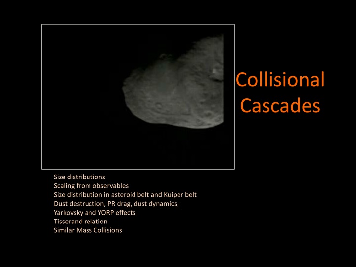
Collisional Cascades Size distributions Scaling from observables Size distribution in asteroid belt and Kuiper belt Dust destruction, PR drag, dust dynamics, Yarkovsky and YORP effects Tisserandrelation Similar Mass Collisions

Power law distributions • Size distribution in terms of radius a • Makes more sense to look at size distribution in log space as that way bins are evenly spaced in log space Can also look at the differential size distribution (integrated up to a) • Mass distribution • Surface area distribution Related to opacity and area filling factor, collision rate. Related to total amount reflected from star or absorbed from star

Scaling from observables • A steady state size distribution in the small end assumed, steady dust production rate • To interpret observed flux, emissivity, opacity and albedo as a function of wavelength for the size distribution must be considered. • For λ < a wavelengths smaller than the particle size, approximate these quantities using particle surface area • For λ > a , emissivity and opacity drop with increasing wavelength • You tend to get information about a ~ λ

Evolution of size distribution • dN(a)/dt = -rate of destruction + rate of production of bodies with radius a • Larger particles destroyed by collisions create smaller particles • Smallest particles can be removed or destroyed by drag, blowout, sputtering, sublimation

Catastrophic impacts • QS amount of energy per unit mass required for catastrophic collision with fragmentation and with largest fragment having at least half the mass of parent. • Q*D amount of energy per unit mass required for catastrophic collision that disperses half of the mass • Q*D>QS for large bodies (larger than about 1km) because self-gravity can hold together a rubble pile • Units J/kg or (cm/s)2 --- set by velocity dispersion Varies as a function of material properties • Popular value of order Q*D~106 erg/g (ice) or a velocity of order 103 cm/s

Catastrophic disruption smaller bodies stronger because they may have fewer flaws self gravity important See O’Brien & Greenberg 2005

Complications and refinements • QS and QD depend on collision angle, impact parameter. Simplest estimates integrate over angle • Fragment kinetic energy and size distribution may be relevant • Power-law forms found by Fujiwara • Asteroids and comets are likely to have a wide range of material properties

Itokawa Rubble pile Lumps and smooth parts, no craters Ida and Dactyl with craters warning: sizes of these objects are not similar

Radial Ratio of impactors • Kinetic energy above that required for catastrophic collision • The ratio of the radii of a body just large enough to catastrophically disrupt another • Insert into KE equation and solve for ε<1

One particle of radius a’ hits another (distribution in a) catastrophically at a rate • The total mass per unit time in particles that are fragmented and become particles at least half this size • So that there is no dependence on a (or mass build up at a higher or low particle radius) a steady state would have size distribution • or for integrated or log distribution q=-2.5 assert that this exponent is zero need log distribution in number (because of ½) mass rate depends on cross section

Mass flux • Mass flux through cascade (from large to small particles) is higher if the velocity dispersion is higher • Mass flux is set by collision rate of largest bodies capable of hitting each other during the lifetime of system. • If the collision timescale of the largest bodies is longer than the age of the system then they don’t enter the cascade • An estimate of the size of the largest particles entering the cascade can be made by setting their collision timescale to the age of the system • Previous assumed destruction rate was independent of a but as Q depends on a, the nature of Q changes the power law index

Single population • If a distribution of one sized body at t=0 • For a single body, the collision rate depends on the number of other bodies • The total number of collisions per unit time depends on the square of the total • Solutions: no grinding until bodies enter cascade, then, total mass and mass flux proportional to t-1

From Dominik & Decin 03

The top of the cascade related to observables, however exponents not precisely known

Complications • As Q*D depends on sizescale. Refinements include taking this into account -> A curve or two power laws instead of one • Actually Q parameter is perhaps only a poor approximation of real parameters which depend on unknown composition • Fragmentation models assumed are often necessarily simplistic • Additional dynamical delivery and removal mechanisms • Assumed no evolution in inclination distribution --- this is probably a bad assumption for debris disks • Recent collisions could affect dust distribution on short timescales. Infrared excess sources could be those in which there were large recent rare collisions (Kenyon and Bromley) though this interpretation has been disputed by statistical studies by Mark Wyatt and others

AsteroidMain Belt Observed size distribution used to constrain material properties O’Brien & Greenberg 05

The size distribution and collision cascade observed constrained by gravitational stirring and other heating processes Figure from Wyatt & Dent 2002 set by age of system scaling from dust opacity

Radiation Forces: PR drag • Relativistic effect leading to slow in-spiral of particles • β Ratio of radiation pressure force compared to gravitational force • Depends on albedo A, luminosity of star L* and is inversely proportional to a (particle radius) • Similar drag force from solar or stellar wind To estimate force replace c with stellar wind velocity, vw, and L* with Debris disks: Those in which the PR drag lifetime is shorter than the age of the system. Implying that production of dust is needed to account for infrared observations. VEGA phenomenon discovery of IRAS satellite.

Dust generated in a ring From Wyatt’s review 08

PR drag, blow out and high eccentricity particles • AU Mic and Beta Pic disks both exhibit a break in surface brightness profiles • Models for this, birth ring with collisions and smaller particles which wind up in eccentric orbits because of radiation pressure • For AU MIC solar wind pressure is a proxy for radiation pressure in Beta Pic Strubbe & Chiang 2006 on AU Mic’s disk

Yarkovskyeffect • Diurnal -- rotating asteroid • dusk side is hotter, so emits more radiation • Relativistic effect causing changes in semi-major axis. • Retrograde rotators spiral inwards • Seasonal • dusk side again hotter, always leading to in-spiraling.

Yarkovsky effect retrograde spin seasonal from Bottke et al. 2006

Yarkovsky effect used for diurnal used for seasonal • penetration depth, ld • K thermal diffusivity, ρ density • Cp specific heat, ε emissivity • ω angular rotation rate • n mean motion • T mean temperature • Θ ratio of cooling time to rotation timescale • If rotation is fast, then Θ is small and whole asteroid is nearly at same temperature, little effect Energy in surface Cooling at a rate Gives a cooling timescale

Yarkovsky effect continued • Radiation pressure depends on the temperature differential ΔT/T~θ • Force is luminosity divided by speed of light or L/c • Total force ~ where A is area • Force per unit mass where R is radius (acceleration) • Enough to estimate da/dt ~ the acceleration divided by the mean motion

Drift Rates of NEOs from main belt The spin period Prot is 6h for bodies larger than 0.15 km in diameter and Prot = 6h × (D/0.15 km) for smaller bodies. Difference between size distributions of NEOs and main belt likely due to this effect O’Brien & Greenberg 06

Yarkovsky effect (continued) • The rotation period is fixed for the seasonal Yarkovsky effect (set by mean motion). For small objects the skin depth maxes at the size of the asteroid. There is a particular sized object that is most affected or has the highest drift rate • For the diurnal Yarkovsky effect, rotations can be different for different sized bodies allowing a broader distribution • Differences not only in NEA and asteroid population size distributions but other phenomena associated with NEA population such as cratering stats

YORP: Yarkovsky–O'Keefe–Radzievskii–Paddack effect • Second order Yakovskyefect • Shape and albedo variations affect both spin rate and rotation axis (obliquity) of asteroids. What we talked about previously affected orbit rather than the spin rate and axis. • Each facet of the asteroid emits light normal to it. Each facet exerts a different torque on the object.

YORP effect • The torque is the acceleration times the radius of the asteroid. • To order of mag one can use the acceleration from the Yarkovsky effect to estimate the acceleration on the surface • Timescale for the YORP effect • Actual timescale would be longer and depend on things like albedo and surface shape

Implications of Yarkovsky and YORP effects • Orbital element evolution in asteroid belt. Dynamical spreading of asteroid families. Resonant feeding rates and meteorite delivery • Size distribution differences between NEO and main belt • Direct measurements with radar: variations in spin, orbital elements

Kuiper Belt size distribution Luminosity function observed for Kuiper Belt • Luminosity distribution is converted to a size distribution. Size distribution is steep with exponent about 4.8 for large bodies but is flatter for small bodies, about 1.9 for smaller bodies • Steep exponent is evidence of runaway accretion • Turn over radius suspected to be due to subsequent collisional evolution if bodies are weak (that means large bodies can be broken up) • No difference observed between high and low inclination objects ruling out different scenarios for them very massive! Break diameter ~50 km From Frazer, W. C. & Kavelaars 2008

Additional dust destructionmechanisms • Sublimation (see Dominik & Decin 03) depends on dust particle temperature • Photo-sputtering (see Grigorieva et al. 07) • UV photons can locally cause grain particles to escape • Sputtering by stellar wind energetic particles (see Mukai & Schwehm 81) • high energy stellar wind particles can cause grain particles to escape – or order 1 particle per solar wind particle, leads to a constant mass flux

Sputtering due to stellar wind particles • Rate proportional to solar wind density, keV particles that can exceed surface binding energy • We can assume the speed is constant so density is proportional to r-2 • For solar wind at radius of Earth sputtering rates are (based on Mukai & Schwem 91) • dM/dtdA ~ 3x10-16g cm-2 s-1 for stony material • dM/dtdA = 4x10-15g cm-2 s-1 for icy material • As we find da/dtis constant • Lifetime is proportional to a t = a/(da/dt) • Sputtering lifetimes can be estimated for other locations and stars by scaling off estimated wind strengths and radius

PR drag in more detail • sw is ratio of solar wind force to radiation pressure • Above is force from Sun, radiation pressure and solar wind forces but neglecting charging of particles radiation pressure relativistic drag

Orbital element evolution due to PR drag • Note if you are reading Liou and Zook’s papers it is customary to work in units of planet’s mean motion and semi-major axis and this includes rescaling the speed of light. Here I have tried to restore units • Timescales for evolution are always • Above predict evolution unless a planet is important

Location of mean motion resonances for small dust particles planet (GM=1) dust particle resonance condition When using orbital element converter work with effective solar mass GM(1-β)

PR drag and resonant capture • If collision time longer than PR drag timescale • Predictions by Liou and Zook that dust in Kuiper belt would be sculpted by resonances with Neptune • Resonant ring captured into resonances with the Earth predicted and observed Image by Wyatt 08

PR drag and resonance capture • Capture probabilities can be computed: Adiabatic limit can be computed as can critical eccentricities. Smaller dust particles which drift faster will be above adiabatic limit for narrow resonances. • Particles are captured into external resonances not internal ones (as expected based on adiabatic capture theory) -------- • Temporary capture in interior resonances seen in simulations but not explained (happens in my toy models if there is a chaotic zone near separatrix) • Little understanding of lifetimes in resonance so constraints on dust production rates only possible from simulations • Ring associated with Mars not yet observed, though it is speculated that even planets as low mass as Mars could be discovered someday from resonant rings (e.g., Stark & Kuchner 08)

Evolution in resonance • It is convenient to consider how PR drag effects the Tisserand relation. • Tisserand relation gives a quantity that is conserved for a particle perturbed by a planet in a circular orbit (related to Jacobi integral). • Gravitational perturbations don’t change the Tisserand relation but PR drag does. This makes it possible to estimate evolution of eccentricity in resonance (Following Liou & Zook 1997) • Remember that in our exploration of first order mean motion resonances we did find a conserved quantity (J2?) which allowed us to reduce the dynamical problem by a dimension.

Jacobi integral • Consider any Hamiltonian with a potential term constant in a rotating frame • Such as the restricted 3 body problem, Sun+ planet in a circular (not eccentric orbit) + massless particle • New Hamiltonian • Jacobi integral written approximately in terms of orbital elements is known as the Tisserand relation New Hamiltonian does not depend on time, so is conserved. -2K is the Jacobi integral

Jacobi integral • Neither energy nor angular momentum were conserved in inertial frame • Jacobi constant or integral is conserved • In non rotating frame • In rotating frame • After coordinate transformation we find that the following is conserved As derived by M+D section 3.3

Jacobi integral in orbital elementsThe Tisserand relation • For a planet • Subbing into Jacobi integral • If we take into account inclination with respect to orbital planet of planet • Let α=a/ap, I inclination w.r.t. planet’s orbit • This is the Tisserand relation, done in limit of low mass planet • Can be used to relate orbital elements before and after an encounter with Jupiter to figure out if a comet is on its first passage through the inner solar system.

Evolution in resonance from Liou & Zook 97 in units of ap consider variations due to just gravity and those due to drag. Insert only PR drag for derivatives as gravity should conserve C. PR drag does not conserve C. Using Tisserand relation search for a steady state with dC/dt=0 but only take into account variations due to PR drag (This is only valid at low e) set K=p/q=a3/2 ( in units of planet’s semi-major axis) equate the two above expressions (one inversed and * -1) and solve for K  each resonance (defined by K) gives a different limiting eccentricity that is the solution to this equation

Evolution in resonance • When e, I small, dC/dt ∝ K-1 – 1 is positive if K <1, negative if K >1 • dC/dt <0 → de/dt >0, dC/dt>0 → de/dt<0 • For external resonances (K>1) eccentricity increases until it reaches the limiting value of e • For internal resonances (K<1) eccentricity drops with time until e=0 then escapes resonance • For K~1 then elim~ 0 • For Large K we have large elim limiting value of eccentricity given by solving this equation The solution to this equation is the eccentricity approached while drifting

Timescale for evolution in resonance • dC/dt only depends on e. Differentiate C and assume da/dt=0 in resonance. Then we can relate dC/dt to de/dt. • Limiting eccentricity approached exponentially --- exp(-3At/K) with and K=p/q>1 • Restoring units a/ap = K2/3 >1 for PR drag

Particle integrations 4micron dust in 2:1 exterior MM resonance with Neptune From Liou &Zook 1997 No clues on what timescale particle escapes from resonance. It can last in resonance indefinitely (meaning as long as I have been willing to integrate) After escape de/dt and da/dt dropping as expected from PR drag alone

Evolution in resonance continued • Larger K means larger final eccentricity • More distant resonances have higher final eccentricity and they evolve more slowly • Limiting eccentricity only depends on K • timescale for evolution only dependent on K and β for limiting eccentricity: evolution timescale: • None of this depends on mass of planet or on order of resonance • Mass of planet does affect capture probabilities and likely to affect resonance lifetimes • Note shift in angle of particle resonance not discussed here! • Angular properties of dust distribution also not discussed here

For other types of drifting For a general dissipation process quadratic equation in β This can be solved for the limiting eccentricity In the limit of high eccentricity damping In the limit of low eccentricity damping lower e high eccentricity e.g., see work by Man-Hoi Lee, Ketchum, Rein on evolution in resonance in multiple planet systems

Eccentricity increase in resonance A captured system can be modeled with b(t) set drift In resonance we take <φ>= constant Hamilton’s equation =0 After capture first two terms dominate  relation between drift rate and rate of eccentricity increase. Rate of eccentricity increase depends on drift rate

Phase angle delay in resonance Hamilton’s equation Relation between drift rate in resonance and phase delay Phase angle offset, predicts an asymmetry that is key to detecting the resonant dust ring with the Earth

Collisions between similar mass bodies • Nearly equal mass collisions are important for: • Diversity of Solar system planets (and possibly extrasolar system planets; Kepler 36) • Moon/Earth collision • Formation of Mercury, accounting for its high density • Moon, Mars hemispheric dichotomy • Obliquities of Uranus, Venus?

Collisional Cascades