Download
1 / 55
550 likes | 652 Views
Concepts of DB(3) Relational Operation & SQL. 한국기술대학교 인터넷미디어공학부 민준기. Relational Data Operation. Procedural language The user instructs the system to perform a sequence of operations on the database to compute the desired result what & how Relational algebra Nonprocedural language

E N D
Concepts of DB(3)Relational Operation & SQL 한국기술대학교 인터넷미디어공학부 민준기
Relational Data Operation • Procedural language • The user instructs the system to perform a sequence of operations on the database to compute the desired result what & how • Relational algebra • Nonprocedural language • The user describes the information desired without a specific procedure for obtaining the information what • Relational calculus • 1.Tuple Relational Calculus • 2.Domain Relational Calculus • Relational Algebra and Relational Calculus have same expression/computing power
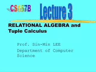
Relational Algebra • Relational Algebra consists of several groups of operations • Relational Algebra Operations From Set Theory • UNION ( ) • INTERSECTION ( ) • DIFFERENCE (or MINUS, – ) • CARTESIAN PRODUCT ( x ) • Relational Operations • Unary Relational Operations • SELECT (symbol: (sigma)) • PROJECT (symbol: (pi)) • RENAME (symbol: (rho)) • Binary Relational Operations • JOIN (several variations of JOIN exist, ) • DIVISION ( ÷ ) • Additional Relational Operations • OUTER JOINS, • OUTER UNION • AGGREGATE FUNCTIONS (These compute summary of information: for example, SUM, COUNT, AVG, MIN, MAX) • closure property • Operand and operation results are relation • Support nested expressions
10 PRODUCT DIVIDE a b c x y a b c x y a a b b c c a a b b c c x y x y x y x y x y x y UNION INTERSECT DIFFERENCE RESTRICTION PROJECTION JOIN a1 a2 a3 b1 b1 b2 b1 b2 b3 c1 c2 c3 a1 a2 a3 b1 b1 b2 c1 c1 c2
Relational Algebra Operations From Set Theory ⅰ. union,∪ R∪S = { t | t∈R ∨ t∈S } |R∪S| ≤ |R| + |S| ⅱ. intersect,∩ R∩S = { t | t∈R ∧ t∈S } |R∩S| ≤ min{ |R|, |S| } ⅲ. difference,- RS = { t | t∈R ∧ t S } |RS| ≤ |R| ⅳ. Cartesian product,× R×S = { r·s | r∈R ∧ s∈S } · : concatenation |R×S| = |R|×|S| degree = R’s degree+ S’s degree
▶Relational Operations • Relation: R(X) = R(A1, ... , An) • R’s tuple r : <a1, ... , an> R={r | r = <a1, ... , an> } • ai : tupler’s attribute Aivalue • ai= r.Ai= r[Ai] • In general, • <r.A1 , r.A2 ,…, r.An > = < r[A1], r[A2], …, r[An] > = r[A1, A2, … An] = r[X]
Unary Relational Operations: SELECT • The SELECT operation (denoted by (sigma)) is used to select a subset of the tuples from a relation based on a selection condition. • The selection condition acts as a filter • Keeps only those tuples that satisfy the qualifying condition • Tuples satisfying the condition are selected whereas the other tuples are discarded (filtered out) horizontal subset Av(R) = { r | r∈R ∧ r.Aθv } AB(R) = { r | r∈R ∧ r.Aθr.B } where, θ(theta) : <, >, ≤, ≥, =, ≠ • Examples: • Select the EMPLOYEE tuples whose department number is 4: DNO = 4 (EMPLOYEE) • Select the employee tuples whose salary is greater than $30,000: SALARY > 30,000 (EMPLOYEE)
Unary Relational Operations: SELECT (contd.) • SELECT Operation Properties • The SELECT operation <selection condition>(R) produces a relation S that has the same schema (same attributes) as R • SELECT is commutative: • <condition1>(< condition2> (R)) = <condition2> (< condition1> (R)) • Because of commutativity property, a cascade (sequence) of SELECT operations may be applied in any order: • <cond1>(<cond2> (<cond3> (R)) = <cond2> (<cond3> (<cond1> ( R))) • A cascade of SELECT operations may be replaced by a single selection with a conjunction of all the conditions: • <cond1>(< cond2> (<cond3>(R)) = <cond1> AND < cond2> AND < cond3>(R))) • The number of tuples in the result of a SELECT is less than (or equal to) the number of tuples in the input relation R • Selectivity
Join • 세타조인 (theta-join) R(X), S(Y), A∈X, B∈Y 에 대하여 R AθB S = { r · s | r∈R ∧ s∈S ∧ ( r.Aθs.B) } • A, B : joining attribute • 결과 차수 = R의 차수 + S의 차수 • example • 학생 학번=학번 등록 • 동일조인 (equi-join) 세타조인에서 θ가 "="인 경우 R A=BS = { r·s | r∈R ∧ s∈S ∧ ( r.A=s.B ) }
Unary Relational Operations: PROJECT • PROJECT Operation is denoted by (pi) • In RelationR(X), ifY⊆X andY={B1,B2, … ,Bm}, Y(R)={ <r.B1, ... , r.Bm> | r∈R } vertical subset • This operation keeps certain columns (attributes) from a relation and discards the other columns. • PROJECT creates a vertical partitioning • The list of specified columns (attributes) is kept in each tuple • The other attributes in each tuple are discarded • Example: To list each employee’s first and last name and salary, the following is used: LNAME, FNAME,SALARY(EMPLOYEE)
Binary Relational Operations: JOIN • JOIN Operation (denoted by ) • The sequence of CARTESIAN PRODECT followed by SELECT is used quite commonly to identify and select related tuples from two relations • A special operation, called JOIN combines this sequence into a single operation • This operation is very important for any relational database with more than a single relation, because it allows us combine related tuples from various relations • The general form of a join operation on two relations R(A1, A2, . . ., An) and S(B1, B2, . . ., Bm) is: R <join condition>S • where R and S can be any relations that result from general relational algebra expressions.
Some properties of JOIN • Consider the following JOIN operation: • R(A1, A2, . . ., An) S(B1, B2, . . ., Bm) R.Ai=S.Bj • Result is a relation Q with degree n + m attributes: • Q(A1, A2, . . ., An, B1, B2, . . ., Bm), in that order. • The resulting relation state has one tuple for each combination of tuples—r from R and s from S, but only if they satisfy the join condition r[Ai]=s[Bj] • Hence, if R has nR tuples, and S has nS tuples, then the join result will generally have less than nR * nS tuples. • Only related tuples (based on the join condition) will appear in the result
Theta JOIN For R(X), S(Y), A∈X, B∈Y , R AθB S = { r · s | r∈R ∧ s∈S ∧ ( r.Aθs.B) } • A, B : join attribute • θ can be any general boolean expression on the attributes of R and S; for example: • R.Ai<S.Bj AND (R.Ak=S.Bl OR R.Ap<S.Bq)
NATURAL JOIN Operation • NATURAL JOIN Operation • Another variation of JOIN called NATURAL JOIN — denoted by N— was created to get rid of the second (superfluous) attribute in an EQUIJOIN condition. • because one of each pair of attributes with identical values is superfluous • natural join: N) If R(X), S(Y)’s join attribute is Z(=X∩Y) R NS = {<r · s>[X∪Y] | r∈R∧s∈S∧r[Z]=s[Z] } = X∪Y(Z=Z(R×S)) = X∪Y(R Z=ZS) • The standard definition of natural join requires that the two join attributes, or each pair of corresponding join attributes, have the same name in both relations
NATURAL JOIN Operation • example: Q R(A,B,C,D) N S(C,D,E) • The implicit join condition includes each pair of attributes with the same name, “AND”ed together: • R.C=S.C AND R.D.S.D • Result keeps only one attribute of each such pair: • Q(A,B,C,D,E)
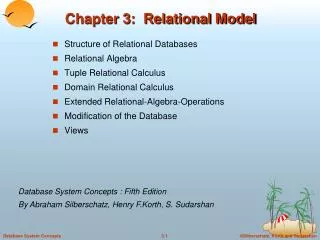
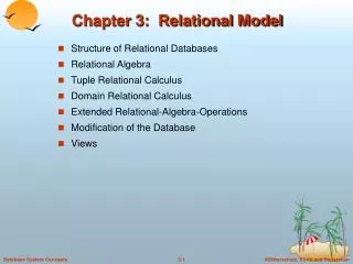
DIVISION: ÷ (1) • DIVISION Operation • The division operation is applied to two relations R(X), S(Y) • R÷S={ t | t∈ D(R) ∧ t · s∈R for all s∈S }, where Y X. Let D = X-Y(and hence X =D Y); that is, let D be the set of attributes of R that are not attributes of S. • The result of DIVISION is a relation T(Y) that includes a tuple t if tuples tR appear in R with tR [Y] = t, and with • tR [X] = tsfor every tuple ts in S. • For a tuple t to appear in the result T of the DIVISION, the values in t must appear in R in combination with every tuple in S. • Note : ((R ÷ S) × S) ⊆ R
학과목(SC) 과목1(C1) 과목2(C2) 과목3(C3) 학번 (SNO) 과목번호 (CNO) 과목번호 (CNO) 과목번호 (CNO) 과목번호 (CNO) 100 C413 C413 C312 C312 100 E412 C413 C413 200 C123 E412 300 C312 300 C324 300 C413 SC ÷ C1 SC ÷ C2 SC ÷ C3 400 C312 400 C324 학번 (SNO) 학번 (SNO) 학번 (SNO) 400 C413 400 E412 100 300 400 500 C312 300 400 400
Extension of Relational Algebra(1) ⅰ. semijoin: • R S: R’s tuples that can be natual join with S • Let R(X), S(Y)’s join attribute beZ(=X∩Y), R S = R N(Z(S)) = X(R NS) • Property • R S ≠ S R • R NS = (R S) NS = (S R) NR
N N N N Natual Join & SemiJoin R S X∩Y(S) R S R S (세미 조인) (자연 조인)
Extension of Relational Algebra(2) • The OUTER JOIN Operation • In NATURAL JOIN and EQUIJOIN, tuples without a matching (or related) tuple are eliminated from the join result • Tuples with null in the join attributes are also eliminated • This amounts to loss of information. • A set of operations, called OUTER joins, can be used when we want to keep all the tuples in R, or all those in S, or all those in both relations in the result of the join, regardless of whether or not they have matching tuples in the other relation. ⅱ. outerjoin, +
Extension of Relational Algebra(3) • The left outer join operation keeps every tuple in the first or left relation R in R S; if no matching tuple is found in S, then the attributes of S in the join result are filled or “padded” with null values. • A similar operation, right outer join, keeps every tuple in the second or right relation S in the result of R S. • A third operation, full outer join, denoted by or + , keeps all tuples in both the left and the right relations when no matching tuples are found, padding them with null values as needed.
N N Natural Join and Outer Join S R + + R S R S (Outer Join) (Natural Join)
Extension of Relational Algebra(4) ⅲ. outer-union, ∪+ • The outer union operation was developed to take the union of tuples from two relations if the relations are not type compatible. • This operation will take the union of tuples in two relations R(X, Y) and S(X, Z) that are partially compatible, meaning that only some of their attributes, say X, are type compatible. • The attributes that are type compatible are represented only once in the result, and those attributes that are not type compatible from either relation are also kept in the result relation T(X, Y, Z).
Outer Union R S ∪+
Extension of Relational Algebra(5) • A type of request that cannot be expressed in the basic relational algebra is to specify mathematical aggregate functions on collections of values from the database. • Examples of such functions include retrieving the average or total salary of all employees or the total number of employee tuples. • These functions are used in simple statistical queries that summarize information from the database tuples. • Common functions applied to collections of numeric values include • SUM, AVERAGE, MAXIMUM, and MINIMUM. • The COUNT function is used for counting tuples or values. • AVGgrade(enroll) • retrieves the average score value from the enroll relation • GROUPyear(student) • Grouping student into subgroups with respect to year • GROUPcnoAVGscore(enroll) • Retrieve the average score of each cnogroup of enroll • General Form: GAFB(E) • E : Relational Algebra expression • F : aggregation fuction( SUM, AVG, MAX, MIN, COUNT) • B : Aggregate attribute • G : GROUP Function • A :Group attribute
▶ Algebra Expression • Retrieve all students’ name and dept sname,dept(student) • Retrieve name and score of a studuent who register C413 course sname,score( cno='C413' (studentNRegister)) • Retrieve name of a professor who teaches ‘database’ profname( cname=‘database'(course))
SQL • SQL • A standard language for RDB • Based on relational algebra and calculus • Features of SQL • No-procedural language • SQL language: handling a set of data satisfying the conditions • Interactive or embedded
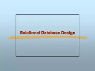
학번 (SNO) 이름 (SNANE) 학년 (YEAR) 학과 (DEPT) 학생 (STUDENT) 100 나 연 묵 4 컴퓨터 200 이 찬 영 3 전기 300 정 기 태 1 컴퓨터 400 송 병 호 4 컴퓨터 500 박 종 화 2 산공 과목번호 (CNO) 과목이름 (CNANE) 학점 (CREDIT) 학과 (DEPT) 담당교수 (PRNAME) 과목 (COURSE) C123 프로그래밍 3 컴퓨터 김성기 C312 자료 구조 3 컴퓨터 황수찬 C324 파일 처리 3 컴퓨터 이규철 C413 데이타 베이스 3 컴퓨터 이석호 C412 반 도 체 3 전자 홍봉희 Sample Table
학번 (SNO) 이름 (SNANE) 학년 (YEAR) 학과 (DEPT) 학생 (STUDENT) 100 나 연 묵 4 컴퓨터 200 이 찬 영 3 전기 300 정 기 태 1 컴퓨터 400 송 병 호 4 컴퓨터 500 박 종 화 2 산공 Basic of SQL • SELECT statement • Retrieve data from table • SELECT clause and FROM clause are mandatory in SELECT statement • WHERE clause is optional to describe the condition SELECT SNAME FROM STUDENT
학번 (SNO) 이름 (SNANE) 학년 (YEAR) 학과 (DEPT) 학생 (STUDENT) 100 나 연 묵 4 컴퓨터 200 이 찬 영 3 전기 300 정 기 태 1 컴퓨터 400 송 병 호 4 컴퓨터 500 박 종 화 2 산공 SQL의 기초 SELECT SNAME FROM STUDENT WHERE YEAR =4
SQL • UNION : • SQL ex: SELECT a FROM R UNION SELECT b FROM S; • INTERSECT : • SQL ex: SELECT a FROM R INTERSECT SELECT b FROM S; • DIFFERENCE : • SQL ex: SELECT a FROM R MINUS SELECT b FROM S; • PRODUCT : • SQL ex: SELECT a, b FROM R, S; • RESTRICTION(SELECTION) : • SQL ex: SELECT * FROM R WHERE r.A=10; • PROJECTION : • SQL ex: SELECT r.A1, r.A2 FROM R; • JOIN • SQL ex: SELECT r.A, r.B FROM R, S WHERE r.A = s.B;
Query Processing • Index • Random data(tuple) access • inefficient • Additional data structure
▶Index method • indexed file consists of • index file • data file Data File Index file address key K1 K2 K3
Traditional Index Structure • B-Tree • B+-Tree
index: (1) B-tree • B-tree (degree = m) • m-way search tree • Except root and leaf, the number of subtrees of internal node is at least ⌈m/2⌉, at most, m • at most, the number of key is ⌈m/2⌉-1 • if root is not a leaf, root has two subtree ats least. • all leaf is same level • balanced tree Note: degree is the maximum number of subtrees
a 69 ^ b c 19 43 128 138 d e f g h i 16 ^ 26 40 60 ^ 100 ^ 132 ^ 145 ^ j k l m n o p q r s t u v 7 15 18 20 30 36 42 50 58 62 65 70 110 120 130 136 140 150 3-naryB-tree
▶ Operation(1) • B-tree • random access: branch by search key • sequential access: in order traversal • Insert/delete: keep balance • split : by node overflow • merge : by node underflow • Insert • Insert done at leaf node • has free space: simple insertion • overflow(no free space) there m keys in a leaf node1) split2) m/2 th key insert parent node3) remains left, right
Example • 59 insert • 57 insert b b f f · · · · · · · 60 ^ 58 60 o o’ o p p · 50 59 50 58 o o’ · 50 57 50
Example • splite by insert 54 • in Parent node f, insert54 o o’ o’’ 54 goes to parent node f · · 50 57 50 57 f f f’ · · · · · · · · · · · ^ ^ 58 60 54 60 58 goes to parent node b o o’ p o o’’ o’ p
b b b’ · · · · · · · · · · · 19 43 19 58 43 goes to parent a d e f d e f f’ Example • parent node b, insert 58 • parent node a, insert 43 ^ ^ a a · · · · · · · ^ 69 43 69 b c b b’ c
▶ Example (2) • Delete • Delete is done at leaf node • Deletion key is not in leaf node • swap with following key • deletion • if # of key< ⌈ m/2 ⌉ -1, underflow • redistribution • sibling node having keys whose number >=⌈m/2⌉ (parent node key → underflow node key) (sibling node key →parent node key) • merge • can not redistribution(sibling node + parent node + underflow node)
Example • delete 60 • delete 20 b b b f f f 60 62 62 o p o p o p 50 50 50 62 65 50 60 65 50 65 b b e e 26 40 30 40 l m n l m n 20 30 36 42 26 36 42
B-Tree insertion(m =5) • Insert 77 72 84 2 7 40 74 75 76 78 89 90 91 Split 72 76 84 2 7 40 74 75 77 78 89 90 91
B-Tree Deletion(m = 5) • Delete 84 72 76 84 2 7 40 74 75 77 78 89 90 91 Swap & Delete 72 76 89 2 7 40 74 75 77 78 84 90 91
B-Tree Deletion • Delete 74 72 76 89 2 7 40 74 75 77 78 90 91 72 76 89 2 7 40 74 75 77 78 90 91 Underflow 발생
B-Tree Deletion Redistribution Using A Adjacent Sibling whose number of key greater than or equal to ceiling(m/2) 72 76 89 2 7 40 74 75 77 78 90 91 {2,7, 40, 72, 75} is redistributed, [m/2] th value(즉, 40) go to parent node 40 76 89 2 7 72 75 77 78 90 91
B-Tree Deleton • Delete 40 40 76 89 2 7 72 75 77 78 90 91 72 76 89 2 7 40 75 77 78 90 91 Swap cannot Redistribution
B-Tree Deletion 72 76 89 2 7 40 75 77 78 90 91 merge with right sibling and parent 72 89 2 7 75 76 77 78 90 91
(2) B+-Tree • B+-tree consists of index set and sequence set 1. index set • consists of internal node • support access path to leaf nodes • support direct access 2. sequence set • consists of leaf nodes • leaf nodes store whole keys support sequential access • leaf node and internal node has different structures
▶ B+-Tree(2) • B+-tree with degree m • node structure<n, P0, K1, P1, K2, P2, … , Pn-1, Kn, Pn> • n : # of keys( 1≤n<m ) • P0, …, Pn :pointer to subtree • K1, …, Kn : key value • root has 0, 2~m subtrees • Except root and leaf, internal node has ⌈m/2⌉~m subtrees • All leaf nodes are same level • key values in nodes is ascending order