Download
1 / 59
590 likes | 755 Views
JCSDA Seminar February 24, 2010. Assimilation of Space-Borne GPS Radio Occultation Data in NWP. Xiaolei Zou Department of Meteorology Florida State University zou@fsu.edu. Outline. Part I: Data (1) Introduction to GPS RO Techniques

E N D
JCSDA Seminar February 24, 2010 Assimilation of Space-Borne GPS Radio Occultation Data in NWP Xiaolei Zou Department of Meteorology Florida State University zou@fsu.edu
Outline Part I:Data (1) Introduction to GPS RO Techniques (2) Data Processing Chain & Error Sources Part II: Assimilation (3) Choices for GPS RO Data Assimilation (4) Highlights of Assimilation Results Part III: Data Application (5)Comparison with Large-Scale Analyses in Cloudy and Clear-Sky Conditions (6) Cloudy Retrieval of GPS RO Data Future Plan
Collaborators • My Ph. D. students & Postdoctoral fellow: H. Shao, L. Lin F. Vandenberghe, B. Wang, H. Liu, Z. Zeng • Ray-tracing model: S. Sokolovskii, M. Gorbunov • Non-local refractivity observation operator: G. Hajj • GPS RO data: R. Anthes, Y.-H. Kuo, M. Exner, D. Hunt, R. Ware, C. Rocken, W. Schreiner, D. Feng, B. Herman
What Is Measured by GPS RO Technique? . A GPS receiver onboard an LEO satellite measures the propagation delay of the radio signals at two L-band frequencies (f1=1.57542 GHz and f2=1.22760 GHz) that are transmitted from a GPS satellite . The propagation delay depends on the distribution of atmospheric refractivity as well as on the ionosphere electron density . The ionosphere effect can be removed by combining the two propagation delays . The wavelengths of the GPS signals are about 20 cm, at which there is very little effect of aerosols, clouds, and rain
, passing through the Earth’s ionosphere and neutral atmosphere, are received at a LEO satellite (~500-2000 km altitude). Instead of being a straight line as in a vacuum, the ray path from GPS (about 20,200 km altitude) to LEO is distorted in the ionosphere and atmosphere, resulting in a small bending. Knowing the precise positions and velocities of the satellites, the total bending (bending angle) can be derived Ray Paths In a vacuum, radio signals travel along straight lines connecting an occulting GPS satellite and LEO satellite. In real atmosphere, any ray path from GPS to LEO satellite is bended in the ionosphere and the atmosphere. The total bending (e.g., bending angle) can be derived given the precise positions and velocities of both satellites.
, passing through the Earth’s ionosphere and neutral atmosphere, are received at a LEO satellite (~500-2000 km altitude). Instead of being a straight line as in a vacuum, the ray path from GPS (about 20,200 km altitude) to LEO is distorted in the ionosphere and atmosphere, resulting in a small bending. Knowing the precise positions and velocities of the satellites, the total bending (bending angle) can be derived Vertical Profiles Due to the satellite motions, the whole atmosphere from top to surface has rays passing through it, obtaining a vertical profile of bending angles from every occurrence of radio occultation. In the lowest ~100 km of the atmosphere, the LEO satellite collects data with a 50 Hzsampling rate, resulting in ~3000 measurements in a vertical profile and a vertical resolution of about 1.5 km in the stratosphere and higher resolution of less than 0.5 km in the lower troposphere. Such an occultation takes about 1 minute.
, passing through the Earth’s ionosphere and neutral atmosphere, are received at a LEO satellite (~500-2000 km altitude). Instead of being a straight line as in a vacuum, the ray path from GPS (about 20,200 km altitude) to LEO is distorted in the ionosphere and atmosphere, resulting in a small bending. Knowing the precise positions and velocities of the satellites, the total bending (bending angle) can be derived Global Coverage There are 24 GPS satellites ((about 20,200 km altitude)in six orbital planes which continuously transmit electro-magnetic waves at two L-band frequencies (f1=1.57542 GHz and f2=1.22760 GHz). With 24 GPS satellites, a single GPS receiver in a near-polar orbit at 800 km will observed over 500 ROs per day, which are distributed fairly uniformly about the globe.
LEO Bending angle α Earth Occulting GPS Atmosphere GPS LEO Earth Atmosphere Bending Angle of a Ray Path Vertical Profiling
COSMIC Anthes et al. 2008 GPS/MET COSMIC II COSMIC SAC-C CHAMP CHAMP SAC-C GPS/MET CHAMP Wickert et al. 2001 GPS/MET GPS/MET Ware et al. 1996; Kursinski et al. 1996 April 2000 Feb. 1997 April 1995 April 2006 SAC-C Hajj et al. 2004 present 2011 present Nov. 2000 present A History of GPS RO Missions 1 LEO 1 LEO 1 LEO 6 LEOs 6~12 LEOs
A Vertical RO Profile from CHAMP Refractivity Bending Angle Measurement Time: 0836UTC 21 May 2002 Averaged Location: (102.04oW, 63.40oS ) Altitude (km) Bending Angle (radian) Refractivity (N unit)
A Vertical RO Profile from CHAMP (cont.) Locations of the tangent points
Data Processing Chain Phase path L1, L2 Excess phase L1, L2 Ionosphere-free excess phase LF Excess Doppler shift fd Bending angle Refractivity N
(1) Phase Path The GPS RO observable is the phase path: where nis the refractive index: N,contribution from the neutral atmosphere ionosphere contribution refractivity
(2) Excess Phase The excess phase is calculated as the difference between the measured phase path and the “vacuum” phase path (equal to the geometric distance between GPS and LEO): where RGL is the geometric distance between GPS and LEO.
Signs of Refractive Index and Excess Phase For microwave frequencies, in the ionosphere and is frequency dependent. in the neutral atmosphere and is independent of frequency. For rays with tangent heights above the tropopause, the excess phase is negative (about 10-100 m) due to the penetration of ionospheric layers on both sides of the neutral atmosphere. The excess phase becomes positive below the tropopause because the effect from the neutral part of the atmosphere exceeds that of the ionosphere. The excessive phase is on the order of 1 km close to the surface.
(3) Removing the Ionosphere Effect Since the first-order contribution of the ionosphere refractivity is inversely proportional to the frequency squared, and can thus be eliminated by applying a linear combination of L1 and L2 at the same time samples: where LF and LF is the ionosphere free phase path and excess phase, respectively.
Magnitude of Excess Phase The ionosphere corrected excess phase, LF is what would be measured had there been no ionosphere at all. Therefore, the ionosphere free excess phase is always positive, and is very small at the high altitude end. In fact, 1 mm at 80 km 1-9 cm at 60 km 1 km at the surface The 1-mm excess phase is less than data noise level.
(4) Excess Doppler Shift The excess Doppler shift is derived as the time derivative of the excess phase: where c is the light velocity in a vacuum.
(5) Bending Angle The excess Doppler shift is related to the satellites geometry: Assuming spherical symmetry: LEO (GPS) is the angle between LEO (GPS) satellite radius and the tangent direction of the LEO (GPS) satellite velocity in the ray plane.
(5) Bending Angle (cont.) Bending angle: Impact parameter:
(6) Refractive Index The Abel inversion: (7) Refractivity
. Error Sources Measurement Errors: (i) Random errors: Clock error and thermal noise (ii) Systematic errors: Signal scattering in the vicinity of the antenna, position errors, velocity errors, and retrieval errors Retrieval errors: Ionosphere calibration errors Upper altitude boundary errors Errors introduced by the spherical symmetry assumption Errors induced by atmospheric multi-path propagation
What to Assimilate? 1. Excessphase: caused by the bending of the radio signal at two frequencies: 1227.6 MHz, 1575.4 MHz. 2. ExcessDoppler frequency shift: estimated by the time derivative of excess phase. 3. Bending angle and impact parameter: derived from Doppler frequency shift based on satellite geometry (impact parameter is assumed constant at GPS and LEO). 4. Refractivity:calculated from bending angle through the Abel inversion (the refractivity is assumed spherically symmetric). 5. Temperature and pressure:retrieved from refractivity using the hydrostatic equation and neglecting water vapor content.
Pros and Cons SSA --- Spheric Symmetry Assumption
(4) Highlights of Assimilation Results (4a) Comparison between bending angle and refractivity assimilation(4b) Comparison between local and non- local refractivity assimilation
Observation Operator for HN FI Interpolate the refractivity onto points along the ray-path where c1=77.6andc2=3.73105 Unit: T (K), q (kg/kg), p (hPa) T,p and q N, N
Observation Operator for H Ray-tracing model: where is the ray trajectory withd=ds/n, s is the length of the ray, and n is the refractivity index. FI HN T,p and q n, n
CHAMP occultations within 6-hr time window centered at 06UTC from 21 to 31 May 2002 Experiment Design NOGPS: Control run BA: Bending angle added to data used in NOGPS REF: Refractivity added to data used in NOGPS Total 434 ROs System:NCEP/SSI T170L42 Data: 03-09 UTC from 21-31 May 2002
Differences in Moisture Analysis Cross-section passing through a CHAMP RO observed at 06 UTC 21 May 2002 RO location: (52.64oN 19.36oW)
Differences in Moisture Analysis (cont.) Zonal variations averaged over all 434 ROs q (g/kg) Grid index
Comparing Three Analyses with CHAMP Refractivity Observations First, Nnon-loc is calculated based on analyses from three data assimilation experiments in the same way as GPS refractivity is derived, i.e., ray-tracing + Abel inversion Second, calculate the mean and standard deviation of the analysis-modeling refractivity from observations, i.e.,
Fractional Mean Altitude (km) Fractional STD NOGAP - CHAMP BA - CHAMP REF - CHAMP Altitude (km)
(4b) Comparison between local and non-local refractivity assimilation
Schematic Illustration of Non-Local Operator Tangent point s Tangent link r Ray path Local curvature center Earth center
Mathematical Expression of Non-Local Operator Approximate the integration along a ray path by its tangent link GPS refractivity (NGPS) is a weighted sum of local refractivity (NLOC) along the tangent link. K is the kernel matrix. Numerical discretization of the two integrals
An Example of K Distribution Vertical resolution is 1 km. Horizontal resolution is 1o. The tangent link is from west to east. The tangent point is located at (0, 30oN).
Practical Implementation GPS Observations: Non-local operator:
700-hPa Refractivity (contour) and Horizontal Gradients (shaded) RO1 in large gradient area RO2 in small gradient area
Differences between Model Simulations and GPS CHAMP Observations RO1 RO2
CloudSat Instrument:94-GHz profiling radar Launch time: April 28, 2006 One orbital time: ~1.5 hours Along-track resolution: ~1.1 km Track width: ~1.4 km reflectivity liquid/ice water content Observed variables: cloud top height cloud base height cloud types
A CloudSat Orbital Track and a Collocated GPS RO Reflectivity (dBz) of a deep convection system One granule of CloudSat orbital track: 17:02:24 UTC June 5, 2007 A collocatedGPS sounding: (72.98oW, 43.79oN)
Vertical Extent of Different Cloud Types High cloud Altostratus Stratocumulus Nimbostratus
Mean/RMS of Fractional N Differences clear-sky 386 ROs Cloudy 1198 ROs ECMWF clear-sky cloudy NCEP 09/2007-08/2008
ECMWF Dependence of Positive N Bias on Cloud Type NCEP High cloud Altostratus Stratocumulus Nimbostratus single-layer cloud only