Download
1 / 56
570 likes | 713 Views
Joint Advanced Student School 2006. Jeff Hillyard Technische Universität München. Magnetic Bearings. Overview Magnetic Bearings. Introduction Magnetism Review Active Magnetic Bearings Passive Magnetic Bearings Industry Applications. Introduction Magnetic Bearing Types.

E N D
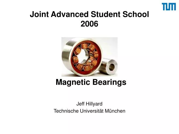
Joint Advanced Student School2006 Jeff Hillyard Technische Universität München Magnetic Bearings
Overview Magnetic Bearings • Introduction • Magnetism Review • Active Magnetic Bearings • Passive Magnetic Bearings • Industry Applications
Introduction Magnetic Bearing Types • Active/passive magnetic bearings • electrically controlled • no control system • Radial/axial magnetic bearings
Introduction Motivations Advantages of magnetic bearings: • contact-free • no lubricant • (no) maintenance • tolerable against heat, cold, vacuum, chemicals • low losses • very high rotational speeds Disadvantages: • complexity • high initial cost Minimum Equipment for AMB Source: Betschon
Introduction Survey of Magnetic Bearings Source: Schweitzer
Magnetism Magnetic Field south pole north pole magnetic field line iron filings Pole Transition
H i Magnetism Magnetic Field Magnetic field, H, is found around a magnet or a current carrying body. (for one current loop)
Magnetism Magnetic Flux Density multiple loops of wire, n B = magnetic flux density • = magnetic permeability H = magnetic field Meissner-Ochsenfeld Effect m0 = permeability of free space mr = relative permeability diamagnetic paramagnetic ferromagnetic
Magnetism B-H Diagram H Ferromagnetic: a material that can be magnetized Remanence, Br magnetic saturation B Coercivity, Hc area within loop represents hysteresis loss
Magnetism Lorentz Force f = force Q = electric charge E = electric field V = velocity of charge Q B = magnetic flux density
Magnetism Lorentz Force Simplification: Source: MIT Physics Dept. website
Magnetism Lorentz Force Further simplification: Analogous Wire B i f force perpendicular to flux!
Magnetism Reluctance Force Force resulting from a difference between magnetic permeabilities in the presence of a magnetic field. force perpendicular to surface! The energy in a magnetic field with linear materials is given by: U = energy V = volume
Aa Magnetism Reluctance Force Basic equation: Energy contained within airgap:
Aa Assumption: Magnetism Reluctance Force Evaluating the magnetic circuit for a simple system:
Magnetism Reluctance Force Principle of virtual displacement: quadratic! 0 inversely quadratic!
Active Magnetic Bearings Elements of System • Electromagnet • Rotor • Sensor • Controller • Amplifier
Active Magnetic Bearings Force Behavior Spring Force Magnetic Force fm fs Force Force xs xs Distance Distance
Active Magnetic BearingsForce Linearization Spring Force Magnetic Force fm fs xs xs
x Active Magnetic BearingsForce Linearization Operating Point (constant current) Redefining distance: fm xs ks = force-displacement factor
im fm fm im im Active Magnetic BearingsForce Linearization Operating Point (constant position) ki = force-current factor
Active Magnetic BearingsForce Linearization im Linearized equation: x Not valid for: • rotor-bearing contact • magnetic saturation • small currents
i x x k d x Active Magnetic BearingsClosed Control Loop Open Loop Equation: Basic System Controller function? - Provide force, f Controller signals? - Input: position, x - Output: current, i i = i(x) Artifical damping and stiffness:
i x x Active Magnetic BearingsClosed Control Loop Solving for controller function: Basic System To model position of rotor: Just like for the spring system!
x(t) t Active Magnetic BearingsClosed Control Loop System characteristics: with General solution for position: Eigenfrequency:
Active Magnetic BearingsClosed Control Loop Controller Abilities: • k, d can be varied in controller • air gap can be varied in controller • specify position for different loads • rotor balancing, vibrations, monitoring...
Active Magnetic BearingsClosed Control Loop Differential driving mode Linearization: magnetic force was determined to be where
Active Magnetic BearingsClosed Control Loop Differential driving mode Linearization: linearized for differential driving mode
Active Magnetic Bearings Bearing Geometry Axial Bearing Radial Bearing
Active Magnetic Bearings Bearing Geometry B circumferential to rotor axis B parallel to rotor axis - similar to electromotors - rotor requires lamination - hysteresis loss low - lamination avoided Orientation: magnet pole pairs are often lined up with the principle coordinate axes x and y (vertical and horizontal) control equations are simplified
sensor + Active Magnetic Bearings Sensors Position Sensor • contact-free • measure rotating surface • surface quality • homogeneity of surface material • various values Other Sensors • speed • current • flux density • temperature • … …other concerns: observability placement cost
Active Magnetic Bearings Sensors “Sensorless“ Bearing - calculate position - less equipment - lower cost Source: Hoffmann
Active Magnetic Bearings Amplifier Converts control signals to control currents. Analog Amplifier: - simple structure - low power applications P<0.6 kVA Switching Amplifier: - lower losses - high power applications - remagnetization loss
Active Magnetic BearingsElectrical Response There is an inherent delay in the electrical system inductance voltage drops: and Total voltage drop: velocity within magnetic field induces a voltage ku = voltage-velocity coefficient
Active Magnetic BearingsControl Equations of Motion Block diagram with voltage control: Source: Schweitzer
Active Magnetic BearingsCurrent vs. Voltage Control Voltage Control: - more accurate model - better stability - low stiffness easier to realize - voltage amplifier often more convenient - possible to avoid using position sensor Current Control: - simple control plant description - simple PD or PID control Flux Control: - very uncommon
Active Magnetic BearingsAddressing of Assumptions Uncertainties in bearing model - leakage flux outside of air gap - air gap is bigger than assumed - iron cross section is non-uniform
Active Magnetic BearingsTypes of Losses Air Losses - air friction divide shaft into sections Copper Losses (Stator) - wire resistance Iron Losses (Rotor) - hysteresis (higher w/ switching amplifier) - eddy currents
Active Magnetic BearingsCopper Losses For differential driving mode: An = slot area Kn = bulk factor r = specific resistance lm = average length of turn limit of permissible mmf!
Active Magnetic BearingsRotor Dynamics Areas of Consideration • natural vibrations • forward/backward whirl (natural vibrations) • critical speeds • nutation • precession (change in rotation axis) Source: Wikipedia
Active Magnetic BearingsRotor Dynamics rotor touch-down in retainer bearings - maintenance - sudden system shutoff - during system shutdown very difficult to simulate cylindrical motion conical motion Source: Schweizer
Active Magnetic Bearings Rotor Stresses Radial Tangential Source: Schweizer largest stress is at inside radius of disc with hole!
Active Magnetic Bearings Rotor Stresses Material vmax (m/s) steel 576 brass 376 bronze 434 aluminium 593 titanium 695 soft ferro. sheets 565 Implications of max stress: max velocity (full disc)! ss = max tensile strength Actual reached speeds (length 600 mm, dia. 45 mm): Source: Schweizer
Passive Magnetic BearingsPermanent Magnets Relative Sizes Common Materials: • neodymium, iron, boron (Nd Fe B) • samarium, cobalt, boron (Sm Co, Sm Co B) • ferrite • aluminium, nickel, cobalt (Al Ni, Al Ni Co) Issues: - material brittleness - varying space requirements (B-H) - operating temperatures (equal H at 10 mm)
Passive Magnetic BearingsPermanent Magnets at least one degree of freedom unstable! reluctance bearings: - non-rotating magnets - resistance to radial displacement increase in stiffness with multiple rings caution: misalignment!
Passive Magnetic BearingsPermanent Magnets High Potential - economical - reliable - practical • already replacing some active magnetic bearings - smaller size equipment and systems - systems with large air gaps Source: Boden
Applications Turbomolecular Pump École Polytechnique Fédérale de Lausanne, Switzerland - eliminates complicated lubrication system - high temperature resistance - reduction of pollution - vibrations, noise, stresses avoided - improved monitoring (unbalances, defects, etc.) Status: suboptimal design • overheating at load (> 550°C) • increase life span • optimize fill factor • reduce cost • simplify manufacturing
Applications Flywheel (‘97) New Energy and Industrial Technology Development Organization (NEDO) – Japan‘s Ministry of International Trade and Industry (MITI) • T=½Jw2 speed has larger influence than mass (better energy density) • fiber-reinforced plastics for high strength • fracture into small pieces upon failure above ground • combination of superconductor and permanent magnet bearings (hsys = 84%)
Applications Flywheel (‘97) Current Development Goals (NEDO) • increase load force • reduce amount load force decrease with time (magnetic flux creep) • reduce rotational loss • increase size of bearings for larger systems
Applications Maglev Trains Maglev = Magnetic Levitation • 150 mm levitation over guideway track • undisturbed from small obstacles (snow, debris, etc.) • typical ave. speed of 350 km/h (max 500 km/h) • what if? Paris-Moscow in 7 hr 10 min (2495 km)! • stator: track, rotor: magnets on train Source: DiscoveryChannel.com