Download
1 / 61
630 likes | 761 Views
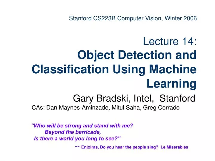
Stanford CS223B Computer Vision, Winter 2006 Lecture 14: Object Detection and Classification Using Machine Learning. Gary Bradski, Intel, Stanford CAs: Dan Maynes-Aminzade, Mitul Saha, Greg Corrado. “Who will be strong and stand with me? Beyond the barricade,

E N D
Stanford CS223B Computer Vision, Winter 2006Lecture 14: Object Detection and Classification Using Machine Learning Gary Bradski, Intel, Stanford CAs: Dan Maynes-Aminzade, Mitul Saha, Greg Corrado “Who will be strong and stand with me? Beyond the barricade, Is there a world you long to see?” -- Enjolras, Do you hear the people sing? Le Miserables
This guy is wearing a haircut called a “Mullet” Fast, accurate and general object recognition …
Find the Mullets… Rapid Learning and Generalization
Approaches to Recognition Geometric Eigen Objects/Turk Shape models Constellation/Perona Patches/Ulman relations MRF/Freeman, Murphy Histograms/Schiele HMAX/Poggio Non-Geo features Local Global We’ll see a few of these …
Eigenfaces Global • Find a new coordinate system that best captures the scatter of the data. • Eigen vectors point in the direction of scatter, ordered of the magnitude of the eigen values. • We can typically prune the number of eigen vectors to a few dozen.
Eigenfaces, the algorithm Global • Assumptions: Square images with W=H=N • M is the number of images in the database • P is the number of persons in the database • The database [slide credit: Alexander Roth]
Eigenfaces, the algorithm Global • Then subtract it from the training faces • We compute the average face [slide credit: Alexander Roth]
Now we build the matrix which is N2by M The covariance matrix which is N2by N2 Eigenfaces, the algorithm Global • Find eigenvalues of the covariance matrix • The matrix is very large • The computational effort is very big • We are interested in at most M eigenvalues • We can reduce the dimension of the matrix [slide credit: Alexander Roth]
Eigenvalue Theorem Global • Define dimension N2 by N2 dimension M by M (e.g., 8 by 8) • Let be an eigenvector of : • Then is eigenvector of : • Proof: This vast dimensionality reduction is what makes the whole thing work. [slide credit: Alexander Roth]
Eigenfaces, the algorithm Global • Eigenvectors of C are linear combination of image space with the eigenvectors of L • Eigenvectors represent the variation in the faces • Compute another matrix which is M by M: • Find the M eigenvalues and eigenvectors • Eigenvectors of C and L are equivalent • Build matrix V from the eigenvectors of L [slide credit: Alexander Roth]
Eigenfaces, the algorithm Global • Compute for each face its projection onto the face space • Compute the between-class threshold [slide credit: Alexander Roth]
Photobook, MIT Example Global Example set Eigenfaces Normalized Eigenfaces [Note: sharper]
Eigenfaces, the algorithm in use Global • To recognize a face, subtract the average face from it • Compute its projection onto the face space • Compute the distance in the face space between the face and all known faces Beyond uses in recognition, Eigen “backgrounds” can be very effective for background subtraction. • Distinguish between • If it’s not a face • If it’s a new face • If it’s a known face [slide credit: Alexander Roth]
Eigenfaces, the algorithm Global • Problemswith eigenfaces – spurious “scatter” • Different illumination • Different head pose • Different alignment • Different facial expression Fisherfaces may beat … • Developed in 1997 by P.Belhumeur et al. • Based on Fisher’s LDA • Faster than eigenfaces, in some cases • Has lower error rates • Works well even if different illumination • Works well even if different facial express. [slide credit: Alexander Roth]
Global/local feature mix Global-noGeo • Global works OK, still used, but local now seems to outperform. • Recent mix of local and global: • Use global features to bias local features with no internal geometric dependencies: Murphy, Torralba & Freeman (03) [image credit: Kevin Murphy]
Use local features to find objects Global-noGeo Filter bank Gaussian within bounding box Image Object bounding box patch Training x positive O negative [image credit: Kevin Murphy]
Global feature: Back to neural nets: Propagate Mixture Density Networks* Global-noGeo Iteration Final output Uses “boostedrandom fields” tolearn graph structure Feature used: Steerable pyramid transformation using 4 orientations and 2 scales; Image divided into 4x4 grid, average energy computed in each channel yields 128 features. PCA down to 80. * C. M. Bishop. Mixture density networks. Technical Report NCRG 4288, Neural Computing Research Group, Department of Computer Science, Aston University, 1994 [slide credit: Kevin Murphy]
Example of context focus Global-noGeo • The algorithm knows where to focus for objects [image credit: Kevin Murphy]
Results Global-noGeo • Performance is boosted by knowing context [image credit: Kevin Murphy]
Completely Local: Color Histograms Local-noGeo • Swain and Ballard ’91 took the normalized r,g,b color histogram of objects: • and noted the tolerance to 3D rotation, partial occlusions etc: [image credit: Swain & Ballard]
Color Histogram Matching Local-noGeo • Objects were recognized based on their histogram intersection: Yielding excellent results over 30 objects: • The problem is, color varies markedly with lighting … [image credit: Swain & Ballard]
Local Feature Histogram Matching Local-noGeo • Scheile and Crowley used derivative type features instead: • And a probabilistic matching rule: • For multiple objects: [image credit: Scheile & Crowley]
Local Feature Histogram Results Local-noGeo • Again with impressive performance results, much more tolerant to lighting: • Problem is: Histograms suffer exponential blow up with number of features 30 of 100f objects [image credit: Scheile & Crowley]
Local Features • Local features, for example: • Lowe’s SIFT • Malik’s Shape Context • Poggio’s HMAX • von der Malsburg’s Gabor Jets • Yokono’s Gaussian Derivative Jets • Adding patches thereof seems to work great, but they are of high dimensionality. • Idea: Encode in Hierarchy: • Overview some techniques...
Convolutional Neural NetworksYann LeCun Local-Hierarchy Broke all the HIPs code (Human Interaction Proofs) from Yahoo, MSN, E-Bay … [image credit: LeCun]
Fragment Based Hierarchy Shimon Ullman Local-Hierarchy • Top down and bottom up hierarchy http://www.wisdom.weizmann.ac.il/~vision/research.html See also Perona’s group work on hierarchical feature models of objects http://www.vision.caltech.edu/html-files/publications.html [image credit: Ullman et al]
Constellation ModelPerona’s Local-Hierarchy • Bayesian Decision based Feature detector results: The shape model. The mean location is indicated by the cross, with the ellipse showing the uncertainty in location. The number by each part is the probability of that part being present. From: Rob Fergus http://www.robots.ox.ac.uk/%7Efergus/ See also Perona’s group work on hierarchical feature models of objects http://www.vision.caltech.edu/html-files/publications.html Recognition Result: The appearance model closest to the mean of the appearance density of each part [image credit: Perona et al]
Joijic and Frey Local-Hierarchy • Scene description as hierarchy of sprites [image credit: Joijic et al]
Jeff Hawkins, Dileep George Local-Hierarchy Results Templates Good Classifications Bad Classifications In (D) Out (E) Hierarchy Module • Modular hierarchical spatial temporal memory [image credit: George, Hawkins]
Peter Bock’s ALISAAn explicit Cognitive Model Local-Hierarchy Histogram based [image credit: Bock et al]
ALISA Labeling 2 Scenes Local-Hierarchy [image credit: Bock et al]
HMAX from the “Standard Model”Maximilian Riesenhuber and Tomaso Poggio Local-Hierarchy In object recognition hierarchy Basic building blocks Modulated by attention Pick this up momentarily, first, a little on trees and boosting … [image credit: Riesenhuber et al]
Machine Learning – Many TechniquesLibraries from Intel Statistical Learning Library: MLL Bayesian Networks Library: PNL focus • Physical Models • Boosted decision trees • MART • Influence diagrams Supervised • SVM • HMM • Multi-Layer Perceptron • BayesNets: Classification • CART • Logistic Regression • Decision trees • K-NN • Radial Basis • Naïve Bayes • Kalman Filter • ARTMAP • Assoc. Net. • Random Forests. • Diagnostic Bayesnet • Bayesnet structure learning • Adaptive Filters • Histogram density est. • Kernel density est. • K-means • Tree distributions • Gaussian Fitting • Dependency Nets • Key: • Optimized • Implemented • Not implemented Unsupervised • ART • Kohonen Map • BayesNets: Parameter fitting • Inference • Spectral clustering • Agglomerative clustering • PCA Modeless Model based
Machine Learning f INPUT OUTPUT underfit f just right y overfit X Learn a model/function That maps input to output • Example Uses of Prediction: • Insurance risk prediction • Parameters that impact yields • Gene classification by function • Topics of a document • . . . Find a function that describes given data and predicts unknown data Specific example: prediction, using a decision tree => => =>
Binary Recursive Decision TreesLeo Breiman’s “CART”* Data of different types, each containing a vector of “predictors” Data set underfit overfit At Each Level: • Find the variable (predictor) and its threshold. • That splits the data into 2 groups • With maximal purity within each group • All variables/predictors are considered at every level. f y maximal purity splits X Perfect purity, but… *Classification And Regression Tree
Binary Recursive Decision TreesLeo Breiman’s “CART”* Data set just right overfit • At Each Level: • Find the variable (predictor) and its threshold. • That splits the data into 2 groups • With maximal purity within each group • All variables/predictors are considered at every level. f y x Prune to avoid over fitting using complexity cost measure
Consider a Face Detector via Decision Stumps Face and non-face data that he features can be tried on Data set It doesn’t detect cars. Bar detector works well for “nose” a face detecting stump. Consider a tree “Stump” – just one split. It selects the single most discriminative feature … For each rectangle combination region: • Find the threshold • That splits the data into 2 groups (face, non-face) • With maximal purity within each group See Appendix for Viola, Jones’s feature generator: Intregral Images maximal purity splits: Thresh = N
We use “Boosting” to Select a “Forest of Stumps” Each stump is a selected feature plus a split threshold Gentle Boost:
For efficient calculation, forma Detection Cascade A boosted cascade is assembled such that at each node, non-object regions stop further processing. If the detection of each node is high (~99.9%), at cost of a high false positive rate (say 50% of everything detected as “object), and if the nodes are independent, Rapid Object Detection using a Boosted Cascade of Simple Features - Viola, Jones (2001)
Improvements to Cascade • J. Wu, J. M. Rehg, and M. D. Mullin just do one Boosting round, then select from the feature pool as needed: • Kobi Levi and Yair Weiss just used better features (gradient histograms) to cut training needs by an order of magnitude. • Let’s focus on better features and descriptors … Viola, Jones Wu, Rehg, Mullin [image credit: Wu et al]
The Standard Model of Visual CortexBiologically Motivated Features .8 .4 .9 .2 .6 • Thomas Serre, Lior Wolf and Tomaso Poggio used the model of the human visual cortex developed in Riesenhuber’s lab: Classifier (SVM, Boosting, …) C2 Layer: Max S2 Response S2 Layer: Radial Basis fit to it’s patch template over the whole image Inter layer: Dictionary of Patches of C1 First 5 chosen features from Boosting C1 layer: Local Spatial Max S1 layer: Gabor at 4 orientations [image credit: Serre et al]
The Standard Model of Visual CortexBiologically Motivated Features • Results in state of the art/top performance: Seems to handily beat SIFT features: [image credit: Serre et al]
Yokonos’ Generalization toThe Standard Model of Visual Cortex • Used Gaussian Derivates: 3 orders X 3 scales X 4 orientations = 36 base features: • Similar to Standard Model’s Gabor base filters. [image credit: Yokono et al]
Yokonos’ Generalization toThe Standard Model of Visual Cortex • Created a local spatial jet, oriented to the gradient at the largest scale at the center pixel: • Since Gabor has ringing spatial extent ~ still approximately similar to standard model. [image credit: Yokono et al]
Yokonos’ Generalization toThe Standard Model of Visual Cortex • Full system: ~S1, C1:Features memorized from positive samples at Harris corner interest points. ~S2:Dictionary of learned features is measured (normalized cross correlation) against all interest points in the image. ~C2:The maximum normalized cross correlation scores are arranged in a feature vector Classifier:Again: SVM, Boosting, … [image credit: Yokono et al]
Yokonos’ Generalization toThe Standard Model of Visual Cortex • Excellent Results: ROC curve for 1200 Stumps: CBCL Database SVM with 1 to 5 training images beats other techniques: [image credit: Yokono et al]
Yokonos’ Generalization toThe Standard Model of Visual Cortex • Excellent Results: Some features chosen: AIBO Dog in articulated poses: ROC Curve: [image credit: Yokono et al]
Brash Claim • In the high 90% performance under lighting, articulation, scale and 3D rotation. • The classifier inside humans is unlikely to be much more accurate. • We are not that far from raw human level performance. • By 2015 I predict. • Base classifier is embedded in larger system that makes it more reliable: • Attention • Color constancy features • Context • Temporal filtering • Sensor fusion
Back to Kevin Murphy: Context: Missing [slide credit: Kevin Murphy]
Context Missing We know there is no keyboard present in this scene … even if there is one indeed. We know there is a keyboard present in this scene even if we cannot see it clearly. [slide credit: Kevin Murphy]