Download
1 / 16
160 likes | 166 Views
Tree-Structured Indexes. Chapter 9. Introduction. As for any index, 3 alternatives for data entries k* : Data record with key value k < k , rid of data record with search key value k > < k , list of rids of data records with search key k >

E N D
Tree-Structured Indexes Chapter 9
Introduction • As for any index, 3 alternatives for data entries k*: • Data record with key value k • <k, rid of data record with search key value k> • <k, list of rids of data records with search key k> • Choice is orthogonal to the indexing technique used to locate data entries k*. • Tree-structured indexing techniques support both range searches and equality searches. • ISAM: static structure;B+ tree: dynamic, adjusts gracefully under inserts and deletes.
Range Searches • ``Find all students with gpa > 3.0’’ • If data is in sorted file, do binary search to find first such student, then scan to find others. • Cost of binary search can be quite high. • Simple idea: Create an `index’ file. Index File kN k2 k1 Data File Page N Page 3 Page 1 Page 2 • Can do binary search on (smaller) index file!
Index Entries (Direct search) Data Entries ("Sequence set") B+ Tree: The Most Widely Used Index • Insert/delete at log F N cost; keep tree height-balanced. (F = fanout, N = # leaf pages) • Minimum 50% occupancy (except for root). • Supports equality and range-searches efficiently.
Example B+ Tree (order p=5, m=4) • Search begins at root, and key comparisons direct it to a leaf (as in ISAM). • Search for 5*, 15*, all data entries >= 24* ... p=5 because tree can have at most 5 pointers in intermediate node; m=4 because at most 4 entries in leaf node. Root 29 7 16 22 39* 3* 5* 19* 20* 22* 24* 27* 38* 2* 7* 14* 16* 29* 33* 34* • Based on the search for 15*, we know it is not in the tree!
B+ Trees in Practice • Typical order: 200. Typical fill-factor: 67%. • average fanout = 133 • Typical capacities: • Height 4: 1334 = 312,900,700 records • Height 3: 1333 = 2,352,637 records • Can often hold top levels in buffer pool: • Level 1 = 1 page = 8 Kbytes • Level 2 = 133 pages = 1 Mbyte • Level 3 = 17,689 pages = 133 MBytes
Inserting a Data Entry into a B+ Tree • Find correct leaf L. • Put data entry onto L. • If L has enough space, done! • Else, must splitL (into L and a new node L2) • Redistribute entries evenly, copy upmiddle key. • Insert index entry pointing to L2 into parent of L. • This can happen recursively • To split index node, redistribute entries evenly, but push upmiddle key. (Contrast with leaf splits.) • Splits “grow” tree; root split increases height. • Tree growth: gets wider or one level taller at top.
Entry to be inserted in parent node. (Note that 17 is pushed up and only 17 this with a leaf split.) 5 13 24 30 Inserting 8* into Example B+ Tree Entry to be inserted in parent node. (Note that 5 is s copied up and • Observe how minimum occupancy is guaranteed in both leaf and index pg splits. • Note difference between copy-upand push-up; be sure you understand the reasons for this. 5 continues to appear in the leaf.) 3* 5* 2* 7* 8* appears once in the index. Contrast
Example B+ Tree After Inserting 8* Root 16 22 3 8 29 39* 2* 3* 5* 7* 8* 19* 20* 22* 24* 27* 38* 29* 33* 34* 14* 16* • Notice that root was split, leading to increase in height. • In this example, we can avoid split by re-distributing entries; however, this is usually not done in practice.
Deleting a Data Entry from a B+ Tree • Start at root, find leaf L where entry belongs. • Remove the entry. • If L is at least half-full, done! • If L has only d-1 entries, • Try to re-distribute, borrowing from sibling (adjacent node with same parent as L). • If re-distribution fails, mergeL and sibling. • If merge occurred, must delete entry (pointing to L or sibling) from parent of L. • Merge could propagate to root, decreasing height.
Example Tree After (Inserting 8*, Then) Deleting 19* and 20* ... • Deleting 19* is easy. • Deleting 20* is done with re-distribution. Notice how middle key is copied up. Root 16 24 3 8 29 39* 2* 3* 5* 7* 8* 22* 24* 27* 29* 38* 33* 34* 14* 16*
... And Then Deleting 24* • Must merge. • Observe `toss’ of index entry (on right), and `pull down’ of index entry (below). 29 39* 22* 27* 38* 29* 33* 34* Root 3 8 16 29 3* 39* 2* 5* 7* 8* 22* 38* 27* 33* 34* 14* 16* 29*
2* 3* 5* 7* 8* 39* 17* 18* 38* 20* 21* 22* 27* 29* 33* 34* 14* 16* Example of Non-leaf Re-distribution • Tree is shown below during deletion of 24*. (What could be a possible initial tree?) • In contrast to previous example, can re-distribute entry from left child of root to right child. Root 21 29 16 18 3 8
After Re-distribution • Intuitively, entries are re-distributed by `pushingthrough’ the splitting entry in the parent node. • It suffices to re-distribute index entry with key 20; we’ve re-distributed 17 as well for illustration. Root 16 3 8 18 21 29 2* 3* 5* 7* 8* 39* 17* 18* 38* 20* 21* 22* 27* 29* 33* 34* 14* 16*
Clarifications B+ Tree • B+ trees can be used to store relations as well as index structures • In the drawn B+ trees we assume (this is not the only scheme) that an intermediate node with q pointers stores the maximum keys of each of the first q-1 subtrees it is pointing to; that is, it contains q-1 keys. • Before B+-tree can be generated the following parameters have to be chosen (based on the available block size; it is assumed one node is stored in one block): • the order p of the tree (p is the maximum number of pointers an intermediate node might have; if it is not a root it must have between round(p/2) and p pointers) • the maximum number m of entries in the leaf node can hold (in general leaf nodes (except the root) must hold between round(m/2) and m entries) • Intermediate nodes usually store more entries than leaf nodes
Summary B+ Tree • Most widely used index in database management systems because of its versatility. One of the most optimized components of a DBMS. • Tree-structured indexes are ideal for range-searches, also good for equality searches (log F N cost). • Inserts/deletes leave tree height-balanced; log F N cost. • High fanout (F) means depth rarely more than 3 or 4. • Almost always better than maintaining a sorted file • Self reorganizing (dynamic data structure) • Typically 67%-full pages at an average