Download
1 / 19
190 likes | 483 Views
. . Introduction. As for any index, 3 alternatives for data entries k*: Data record with key value k <k, rid of data record with search key value k> <k, list of rids of data records with search key k>Choice is orthogonal to the indexing technique used to locate data entries k*.Tree-structured i

E N D
1. Tree-Structured Indexes The slides for this text are organized into chapters. This lecture covers Chapter 9.
Chapter 1: Introduction to Database Systems
Chapter 2: The Entity-Relationship Model
Chapter 3: The Relational Model
Chapter 4 (Part A): Relational Algebra
Chapter 4 (Part B): Relational Calculus
Chapter 5: SQL: Queries, Programming, Triggers
Chapter 6: Query-by-Example (QBE)
Chapter 7: Storing Data: Disks and Files
Chapter 8: File Organizations and Indexing
Chapter 9: Tree-Structured Indexing
Chapter 10: Hash-Based Indexing
Chapter 11: External Sorting
Chapter 12 (Part A): Evaluation of Relational Operators
Chapter 12 (Part B): Evaluation of Relational Operators: Other Techniques
Chapter 13: Introduction to Query Optimization
Chapter 14: A Typical Relational Optimizer
Chapter 15: Schema Refinement and Normal Forms
Chapter 16 (Part A): Physical Database Design
Chapter 16 (Part B): Database Tuning
Chapter 17: Security
Chapter 18: Transaction Management Overview
Chapter 19: Concurrency Control
Chapter 20: Crash Recovery
Chapter 21: Parallel and Distributed Databases
Chapter 22: Internet Databases
Chapter 23: Decision Support
Chapter 24: Data Mining
Chapter 25: Object-Database Systems
Chapter 26: Spatial Data Management
Chapter 27: Deductive Databases
Chapter 28: Additional Topics
The slides for this text are organized into chapters. This lecture covers Chapter 9.
Chapter 1: Introduction to Database Systems
Chapter 2: The Entity-Relationship Model
Chapter 3: The Relational Model
Chapter 4 (Part A): Relational Algebra
Chapter 4 (Part B): Relational Calculus
Chapter 5: SQL: Queries, Programming, Triggers
Chapter 6: Query-by-Example (QBE)
Chapter 7: Storing Data: Disks and Files
Chapter 8: File Organizations and Indexing
Chapter 9: Tree-Structured Indexing
Chapter 10: Hash-Based Indexing
Chapter 11: External Sorting
Chapter 12 (Part A): Evaluation of Relational Operators
Chapter 12 (Part B): Evaluation of Relational Operators: Other Techniques
Chapter 13: Introduction to Query Optimization
Chapter 14: A Typical Relational Optimizer
Chapter 15: Schema Refinement and Normal Forms
Chapter 16 (Part A): Physical Database Design
Chapter 16 (Part B): Database Tuning
Chapter 17: Security
Chapter 18: Transaction Management Overview
Chapter 19: Concurrency Control
Chapter 20: Crash Recovery
Chapter 21: Parallel and Distributed Databases
Chapter 22: Internet Databases
Chapter 23: Decision Support
Chapter 24: Data Mining
Chapter 25: Object-Database Systems
Chapter 26: Spatial Data Management
Chapter 27: Deductive Databases
Chapter 28: Additional Topics
2. Introduction As for any index, 3 alternatives for data entries k*:
Data record with key value k
<k, rid of data record with search key value k>
<k, list of rids of data records with search key k>
Choice is orthogonal to the indexing technique used to locate data entries k*.
Tree-structured indexing techniques support both range searches and equality searches.
ISAM: static structure; B+ tree: dynamic, adjusts gracefully under inserts and deletes.
3. Range Searches ``Find all students with gpa > 3.0��
If data is in sorted file, do binary search to find first such student, then scan to find others.
Cost of binary search can be quite high.
Simple idea: Create an `index� file.
4. ISAM Index file may still be quite large. But we can apply the idea repeatedly!
5. Comments on ISAM File creation:
Leaf (data) pages allocated sequentially, sorted by search key;
then index pages allocated, then space for overflow pages.
Index entries: <search key value, page id>; they `direct� search for data entries, which are in leaf pages.
Search: Start at root; use key comparisons to go to leaf. Cost log F N ; F = # entries/index pg, N = # leaf pgs
Insert: Find leaf data entry belongs to, and put it there.
Delete: Find and remove from leaf; if empty overflow page, de-allocate.
6. Example ISAM Tree Each node can hold 2 entries; no need for `next-leaf-page� pointers.
7. After Inserting 23*, 48*, 41*, 42* ...
8. ... Then Deleting 42*, 51*, 97*
9. B+ Tree: The Most Widely Used Index Insert/delete at log F N cost; keep tree height-balanced. (F = fanout, N = # leaf pages)
Minimum 50% occupancy (except for root). Each node contains d <= m <= 2d entries. The parameter d is called the order of the tree.
Supports equality and range-searches efficiently.
10. Example B+ Tree Search begins at root, and key comparisons direct it to a leaf (as in ISAM).
Search for 5*, 15*, all data entries >= 24* ...
11. B+ Trees in Practice Typical order: 100. Typical fill-factor: 67%.
average fanout = 133
Typical capacities:
Height 4: 1334 = 312,900,700 records
Height 3: 1333 = 2,352,637 records
Can often hold top levels in buffer pool:
Level 1 = 1 page = 8 Kbytes
Level 2 = 133 pages = 1 Mbyte
Level 3 = 17,689 pages = 133 MBytes
12. Inserting a Data Entry into a B+ Tree Find correct leaf L.
Put data entry onto L.
If L has enough space, done!
Else, must split L (into L and a new node L2)
Redistribute entries evenly, copy up middle key.
Insert index entry pointing to L2 into parent of L.
This can happen recursively
To split index node, redistribute entries evenly, but push up middle key. (Contrast with leaf splits.)
Splits �grow� tree; root split increases height.
Tree growth: gets wider or one level taller at top.
13. Inserting 8* into Example B+ Tree Observe how minimum occupancy is guaranteed in both leaf and index pg splits.
Note difference between copy-up and push-up; be sure you understand the reasons for this.
14. Example B+ Tree After Inserting 8*
15. Deleting a Data Entry from a B+ Tree Start at root, find leaf L where entry belongs.
Remove the entry.
If L is at least half-full, done!
If L has only d-1 entries,
Try to re-distribute, borrowing from sibling (adjacent node with same parent as L).
If re-distribution fails, merge L and sibling.
If merge occurred, must delete entry (pointing to L or sibling) from parent of L.
Merge could propagate to root, decreasing height.
16. Example Tree After (Inserting 8*, Then) Deleting 19* and 20* ... Deleting 19* is easy.
Deleting 20* is done with re-distribution. Notice how middle key is copied up.
17. ... And Then Deleting 24* Must merge.
Observe `toss� of index entry (on right), and `pull down� of index entry (below).
18. Summary Tree-structured indexes are ideal for range-searches, also good for equality searches.
ISAM is a static structure.
Only leaf pages modified; overflow pages needed.
Overflow chains can degrade performance unless size of data set and data distribution stay constant.
B+ tree is a dynamic structure.
Inserts/deletes leave tree height-balanced; log F N cost.
High fanout (F) means depth rarely more than 3 or 4.
Almost always better than maintaining a sorted file.
19. Summary (Contd.) Typically, 67% occupancy on average.
Usually preferable to ISAM, modulo locking considerations; adjusts to growth gracefully.
Key compression increases fanout, reduces height.
Bulk loading can be much faster than repeated inserts for creating a B+ tree on a large data set.
Most widely used index in database management systems because of its versatility. One of the most optimized components of a DBMS.