Download
1 / 27
310 likes | 516 Views
Multimedia Data The DCT and JPEG Image Compression. Dr Mike Spann http://www.eee.bham.ac.uk/spannm M.Spann@bham.ac.uk Electronic, Electrical and Computer Engineering. Contents. The philosophy behind the lossy of processes of DCT image compression.

E N D
Multimedia DataTheDCT and JPEG Image Compression Dr Mike Spann http://www.eee.bham.ac.uk/spannm M.Spann@bham.ac.uk Electronic, Electrical and Computer Engineering
Contents • The philosophy behind the lossy of processes of DCT image compression. • A summary of the processes involved in DCT image compression. • Consideration of DCT ringing and blocking compression artefacts; their appearance and their origin.
Lossy DCT Image Compression • The lossy (Discrete Cosine Transform) DCT method compression method is widely used in current standards. For example, JPEG images and MPEG-1 and MPEG-2 (DVD) videos. • The image here is increasingly compressed from left to right. • Blockingartefacts are visible. Ringing artefacts can also be seen around edges. • This lecture will explain how the method works and how these artefacts are caused.
Rate/Distortion a) Original b) CR 8:1 c) CR 11.6:1 d) CR 13.6:1 e) CR 14.2:1 f) Difference a-e g) CR=8:1 with Channel Error • As we have seen, quality can fall rapidly as shown by the steep slope of rate/ distortion graph. • The DCT methods typically* work well up to around 10:1 compression ratios and then quality falls rapidly beyond this. *Note – the original quality and image type are important considerations.
DCT Image Compression • The philosophy behind DCT image compression is that the human eye is less sensitive to higher-frequency information and also more sensitive to intensity than to colour. • The examples here show the effects of percentage reduction of colour by spatially sub-sampling the colour (UV) channels
DCT Image Compression • The DCT method is an example of a transform method. Rather than simply trying to compress the pixel values directly, the image is first TRANSFORMED into the frequency domain. Compression can now be achieved by more coarsely quantizing the large amount of high-frequency components usually present. • The JPEG* standard algorithm for full-colour and grey-scale image compression is a DCT compression standard that uses 8x8 blocks. • It was not designed for graphics or line drawings and is not suited to these image types. *Joint [CCITT and ISO] Photographic Experts Group
DCT Image Compression • The Discrete Cosine Method uses continuous cosine waves, like cos(x) below, of increasing frequencies to represent the image pixels. • The bases are the set of 64 frequencies that can be combined to represent each block of 64 pixels. • Firstly, the image must be transformed into the frequency domain. This is done in blocks across the whole image.
The Discrete Cosine Transform Bases Low frequency High frequency
The DCT • Take each 8x8 pixel block and represent it as amounts (coefficients) of the basis functions (the frequency set). • represent the 8x8 pixels as amounts of lowest frequency (the average or DC value) through to the highest frequency • 64 pixels values are TRANSFORMED into 64 coefficients which represent the amount of each frequency.
DCT Image Compression • The DCT itself does not achieve compression, but rather prepares the image for compression. • Once in the frequency domain the image's high-frequency coefficients can be coarsely quantised so that many of them (>50%) can be truncated to zero. • The coefficients can then be arranged so that the zeroes are clustered (zig-zag collection) and Run-Length Encoded. • The remaining data is then compressed with Huffman coding*. • *The JPEG standard actually specifies many variants which have not been widely used. For example, a more efficient algorithm than Huffman, called arithmetic coding, is a standard variant, but there are several patents on this method. We usually refer to the JPEG baseline algorithm if there is a possibility of confusion between variants.
DCT Image Compression • ‘Baseline’ JPEG uses a standard quantization matrix - determined by subjective testing • Higher frequency DCT coefficients Gijare attenuated more as the HVS is less sensitive to high frequencies 16 11 10 16 24 40 51 61 12 12 14 19 26 58 60 55 14 13 16 24 40 57 69 56 14 17 22 29 51 87 80 62 18 22 37 56 68 109 103 77 24 35 55 64 81 104 113 92 49 64 78 87 103 121 120 101 72 92 95 98 112 100 103 99 Q =
DCT Compression Stages • Blocking (8x8) • DCT (Discrete Cosine Transformation) • Quantization • Zigzag Scan • DPCM* on the dc value (the average value in the top left) • DPCM – Differential Pulse Code Modulation – Instead of sending the value send the difference from the previous value. • RLE on the ac values (all 63 values which aren’t the dc/ average) • Huffman Coding
DCT Mathematics • The formula is shown here for interest only (not assessed material!). • The Discrete Cosine Transform below takes the image pixels I(x,y) and generates DCT(i,j) values. • Its easy to go in the opposite direction as shown in the second equation
Gibb’s Phenomenon • The presence of artefacts around sharp edges is referred to as Gibb's phenomenon. • These are caused by the inability of a finite combination of continuous functions (like cosines) to describe jump discontinuities (e.g. edges). • At higher compression ratios these losses become more apparent, as do the boundaries of the 8x8 blocks. • The loss of edge clarity can be clearly seen in a difference mapping comparing an original image with its heavily compressed equivalent. http://www.numerit.com/samples/fours/doc.htm
Original Test ImageAn extreme example for demonstrating Gibb’s phenomenon
Summary of DCT • The philosophy behind the lossy processes of DCT image compression. • A summary of the processes involved in DCT image compression. • Consideration of DCT ringing and blocking compression artefacts; their appearance and their origin. For interest … more links on compression … http://www.eee.bham.ac.uk/woolleysi/links/datacomp.htm
State of the art compression methods • The DCT is the transformation underpinning the original JPEG standard • Block based transformation • Blocking artefacts will always be an issue at high compression rates • JPEG2000 is based on the discrete wavelettransform (DWT) • A more complex transformation across the whole image • Blocking artefacts no longer a problem DWT
State of the art compression methods • Performance of wavelet based methods is impressive • This is in terms of the quality of the compressed image at high compression rates AND • The absence of blocking artefacts • We can compare DCT and DWT based compression at 32:1 compression ratio DCT DWT
State of the art compression methods • Its much easier to see a difference if we ‘zoom in’ on a small region • Blocking artefacts are clearly visible in the DCT based method • Wavelet based methods ‘degrade’ much more gracefully at higher compression ratios DCT DWT
State of the art compression methods • Another advantage of these methods is that it produces an ‘embedded’ bitstream • Important for video streaming services • The image can be reconstructed from the bitstream at any time according to the quality required at any given compression bitstream ….1100101011100101100011………01011100010111011011101101…. lossless
This concludes our introduction to DCT image compression. • You can find course information, including slides and supporting resources, on-line on the course web page at Thank You http://www.eee.bham.ac.uk/spannm/Courses/ee1f2.htm