Download
1 / 77
770 likes | 928 Views
Lecture 2-5: repeated measurements. Dishman , R. (2008) Gene–Physical Activity Interactions in the Etiology of Obesity: Behavioral Considerations. Obesity, 16: S60-S65. Objectives . Understand: Multilevel data Random vs. fixed effects ICC Choose between

E N D
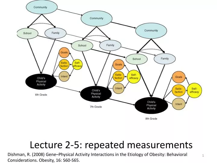
Lecture 2-5: repeated measurements Dishman, R. (2008) Gene–Physical Activity Interactions in the Etiology of Obesity: Behavioral Considerations. Obesity, 16: S60-S65.
Objectives • Understand: • Multilevel data • Random vs. fixed effects • ICC • Choose between • Mixed linear models vs. repeated measures ANOVA
Definition: multilevel data • Data can be non-independent for various reasons: • Clustered in groups (children in classes) • Several measures from same individual • Conditions while taking the measures (e.g., half of them taken in the morning, half in the afternoon)
Other examples from your lab • Clinical: Time within subject within therapist • Social: participants within RA within days • Business: pre-post within individuals within media market
Comparing more than 2 means: Analysis of variance or ANOVA • Null hypothesis: 1 = 2 = 3 =… • If the test is non-significant (p>0.05), we do not reject the null hypothesis that all means are equal (1 = 2 = 3 =…) • If the test is significant (p<0.05), we reject the null hypothesis that all mean are equal (1 = 2 = 3 =…)
Vocabulary • Factors • Variables • Levels / categories / stratum • Cells (a single combination of all the categorical IV) • Main effects (unique effect of one IV) • Simple effects (unique effect of one IV at one level of another IV) • Interaction effects (combined effect of multiple IV)
Why is it called “analysis of variance” • We separate the variance into two components: • Variance within groups • Variance between groups • If the between variance is larger than the within variance, we reject the null hypothesis • Test statistic: F, with 2 types of degree of freedom: M: groups – 1 N: observations – M groups
= + = + Vartot MStot Varbetween MSbetween Varwithin MSwithin Partition of the variance • Variance: + We separate the sum of squares among the between and within, and we do the same for the DF. However, the variance cannot be divided similarly into two parts.
Conditions of application • Independence of observations • Normality within each group (conditional normality) • Robust to violations so long as populations are symmetrical or similarly asymmetrical • Homogeneity of variance • Robust to violations so long as • Largest variance is not more than 4x smallest variance • Group sample sizes are approximately equal
Contrasts • Allow to test specific patterns in group effects • But… • They can be significant when the data do not fit your hypothesized pattern • Some data get ignored • They encourage researchers to “fish” (and you will finally get something) • Be careful what you wish for because you may get it
How to correct for multiple tests: A priori contrasts (planned) • Usually done by ANOVA (all contrasts within a single ANOVA, but could be done by study, or by database,…) • Multiple (also called pairwise) comparisons • Bonferroni (Dunn’s test): a’=a/c (c=# comparison)Perneger, T.V. (1998). What is wrong with Bonferroni adjustments. BMJ, 136, 1236-1238. • Dunn-Sidak: a’=1-(1-a)1/c • Holm test: do the first test using Bonferroni correction (a’=a/c), the next one with c-1, and so on… • Fisher’s LSD: If F is nonsignificant, do not do contrastsif F is significant, make pairwise comparison, using t-test but replacing SD by MSwithin • Scheffe, Tukey, … • False discovery rate (FDR): when you have many tests, expected proportion of false rejections to total rejections
Post-hoc and subgroup analyses • http://www.economist.com/node/8733754?story_id=8733754
Total sum of squares dftotal= N-1 = 25-1 = 24
Between-group sum of squaresalso called SSgroup and SStreatment dfbetween= k-1 = 5-1 = 4
Within-group sum of squaresalso called SSerror and SSresiduals dfwithin= k(n-1) = N-k = 25-5 = 20
How to determine whether an IV is fixed or random • Are the level of the IV chosen in a planned manner? • Or were they randomly selected among other possible instances?
Example: semantic priming data • Subjects had to decide as quickly as possible whether a target (object’s drawing) appearing after a primer (action of a pantomime) was a real object or not. The delay between the pantomime and the apparition of the target was either short or long, the pantomime was of one of three types (related, neutral, or unrelated). The response is the average time to decide if the object is real or not between five measures (without first trial and the errors)
Question • What is the DV? • What are the IV? For each IV, random or fixed? • For each IV, repeated or not? • What is N? • What is n by cell?
Model: semantic data • Yijk ~ a,bjXj, bkXk,b3XjXk,si,eijk • Where a is the overall mean • bjXj is the mean effect due to level j of the factor delay on the mean response • bkXk is the mean effect due to level k of the factor type on the mean response • b3XjXk is the mean effect due to the interaction of level j of the factor delay and level k of the factor type on the mean response
Model: semantic data • Yijk ~ a,bjXj, bkXk,b3XjXk,si,eijk • si is the random effect due to subject i on the mean response and is supposed iid as N(0; s2s) (i = 1; … ; 21), • And eijk is the residual error and is supposed iid as N(0, s2e) • Cov(si,eijk) = 0
Question: semantic data • Present the full regression equation for the semantic data • Yijk = a +b1Xj + b2Xk1+b3Xk2+b4XjXk1+b5XjXk1 + u0i + eijk • Where Xj is delay coded 0 for short and 1 for long • Xk1 is a dummy variable coded 0 for unrelated and related and 1 for neutral • Xk2is a dummy variable coded 0 for unrelated and neutral and 1 for related • u0i is a random intercept that has a different value for each individual i but with mean 0
Model: semantic data • This model assumes that the effect of the subject (si) is the same across all combinations of j and k. • Could the subject effect depend on the levels of one or both factors (e.g., the difference between subjects at one level of one factor is not the same as the difference between subjects at another level of the same factor). • Question: for these data, are those effects estimable?
When is an effect not estimable • When there is only one observation for a combination of cells… • Why? • Because the effect is indistinguishable from residual/individual variability
From ANOVA to regression: mathematically • Yi = a+b1X1+b2X2+…+ei • When the IV are continuous, b is a slope (regression coefficient) • When the IV are categorical, b is a mean difference between the reference and the other category • What is the reference? • What happens when the IV is categorical but there are more than two levels? • Dummy coding
Repeated measures ANOVA • Condition of application: • Compound symmetry (the covariances of conditions are identical)
Repeated measures ANOVA • Condition of application: • Sphericity (the variances of the difference of each pair of conditions are identical)
RM ANOVA: condition of application • If compound symmetry is met, OK • If not, then test sphericity (e is an estimate of sphericity, range 0-1 with 1 = sphericity met) • If sphericity not OK, • you could do a MANOVA (i.e., treat each condition as a DV and look at all the DVs together) • You could correct for sphericity (this in fact corrects the df). Best practice: • e>.75, use Huynh-Feldt correction • e<.75, use Greenhouse-Geisser correction
Limitations of RM ANOVA • Number of observations by cell have to be equal (even one missing data means all observations for this subject are useless) • Number of cells have to be equal (for subjects) • Compound symmetry or sphericity assumption • What do these assumptions mean from a substantive point of view?
X Y Z Confounding variable Confounding X Y
3 levels of Z 3 levels of Z Y Y X X X and Y are not associated within each level of Z X and Y are associated within each level of Z Confounding
Mediation: Baron and Kenny 1986 • There must be a significant relationship between the independent variable and the dependent variable, • There must be a significant relationship between the independent variable and the mediating variable, and • The mediator must be a significant predictor of the outcome variable in an equation including both the mediator and the independent variable. MacKinnon, D. P., Krull, J. L., Lockwood, C. M. (2000). Equivalence of the mediation, confounding and suppression effect. Prevention Science. 1(4). 173-181.
Moderation and interaction • A variable moderates another when the association between the IV and the DV is different for one level of the moderator variable than for another level. • Example: the effect of antibiotics on response time is very small for people not drinking alcohol but is large for people drinking alcohol (alcohol is the moderator variable) • “The difference in response time due to antibiotics differs across alcohol level” • 2 different in the sentence
Be careful about: • Power: if you want to test a hypothesis about a moderator, the necessary sample size is very high. • Interaction may be due to floor or ceiling effect • Interpreting the main effect when there is aninteraction
How to proceed • Look at interaction plots • Estimate the interaction effect • If significant: • Estimate simple effects (relationship between IV and DV for a specific level of a third (moderator) variable)
Example: effect of a stress management course on policemen violence in different districts