Download
1 / 53
540 likes | 636 Views
I/O Introduction: Storage Devices, Metrics. Motivation: Who Cares About I/O?. CPU Performance: 60% per year I/O system performance limited by mechanical delays (disk I/O) < 10% per year (IO per sec or MB per sec) Amdahl's Law: system speed-up limited by the slowest part!

E N D
Motivation: Who Cares About I/O? • CPU Performance: 60% per year • I/O system performance limited by mechanical delays (disk I/O) < 10% per year (IO per sec or MB per sec) • Amdahl's Law: system speed-up limited by the slowest part! 10% IO & 10x CPU => 5x Performance (lose 50%) 10% IO & 100x CPU => 10x Performance (lose 90%) • I/O bottleneck: Diminishing fraction of time in CPU Diminishing value of faster CPUs
Storage System Issues • A Little Queuing Theory • Redundant Arrarys of Inexpensive Disks (RAID) • I/O Buses • I/O Benchmarks
I/O Systems interrupts Processor Cache Memory - I/O Bus Main Memory I/O Controller I/O Controller I/O Controller Graphics Disk Disk Network
Technology Trends Disk Capacity now doubles every 18 months; before 1990 every 36 motnhs • Today: Processing Power Doubles Every 18 months • Today: Memory Size Doubles Every 18 months(4X/3yr) • Today: Disk Capacity Doubles Every 18 months • Disk Positioning Rate (Seek + Rotate) Doubles Every Ten Years! The I/O GAP
Alternative Data Storage Technologies: Early 1990s Cap BPI TPI BPI*TPI Data Xfer Access Technology (MB) (Million) (KByte/s) Time Conventional Tape: Cartridge (.25") 150 12000 104 1.2 92 minutes IBM 3490 (.5") 800 22860 38 0.9 3000 seconds Helical Scan Tape: Video (8mm) 4600 43200 1638 71 492 45 secs DAT (4mm) 1300 61000 1870 114 183 20 secs Magnetic & Optical Disk: Hard Disk (5.25") 1200 33528 1880 63 3000 18 ms IBM 3390 (10.5") 3800 27940 2235 62 4250 20 ms Sony MO (5.25") 640 24130 18796 454 88 100 ms
Response time = Queue + Controller + Seek + Rot + Xfer Service time Devices: Magnetic Disks Track Sector • Purpose: • Long-term, nonvolatile storage • Large, inexpensive, slow level in the storage hierarchy • Characteristics: • Seek Time (~8 ms avg) • positional latency • rotational latency • Transfer rate • About a sector per ms (5-15 MB/s) • Blocks • Capacity • Gigabytes • Quadruples every 3 years (aerodynamics) Cylinder Platter Head 7200 RPM = 120 RPS => 8 ms per rev ave rot. latency = 4 ms 128 sectors per track => 0.25 ms per sector 1 KB per sector => 16 MB / s
Disk Device Terminology Disk Latency = Queuing Time + Controller time + Seek Time + Rotation Time + Xfer Time Order of magnitude times for 4K byte transfers: Seek: 8 ms or less Rotate: 4.2 ms @ 7200 rpm Xfer: 1 ms @ 7200 rpm
Tape vs. Disk • • Longitudinal tape uses same technology as • hard disk; tracks its density improvements • Disk head flies above surface, tape head lies on surface • Disk fixed, tape removable • • Inherent cost-performance based on geometries: • fixed rotating platters with gaps • (random access, limited area, 1 media / reader) • vs. • removable long strips wound on spool • (sequential access, "unlimited" length, multiple / reader) • • New technology trend: • Helical Scan (VCR, Camcoder, DAT) • Spins head at angle to tape to improve density
Current Drawbacks to Tape • Tape wear out: • Helical 100s of passes to 1000s for longitudinal • Head wear out: • 2000 hours for helical • Both must be accounted for in economic / reliability model • Long rewind, eject, load, spin-up times; not inherent, just no need in marketplace (so far) • Designed for archival
Relative Cost of Storage Technology—Late 1995/Early 1996 Magnetic Disks 5.25” 9.1 GB $2129 $0.23/MB $1985 $0.22/MB 3.5” 4.3 GB $1199 $0.27/MB $999 $0.23/MB 2.5” 514 MB $299 $0.58/MB 1.1 GB $345 $0.33/MB Optical Disks 5.25” 4.6 GB $1695+199 $0.41/MB $1499+189 $0.39/MB PCMCIA Cards Static RAM 4.0 MB $700 $175/MB Flash RAM 40.0 MB $1300 $32/MB 175 MB $3600 $20.50/MB
Queue Proc IOC Device Disk I/O Performance Response Time (ms) 300 Metrics: Response Time Throughput 200 100 0 100% 0% Throughput (% total BW) Response time = Queue + Device Service time
Disk Time Example • Disk Parameters: • Transfer size is 8K bytes • Advertised average seek is 12 ms • Disk spins at 7200 RPM • Transfer rate is 4 MB/sec • Controller overhead is 2 ms • Assume that disk is idle so no queuing delay • What is Average Disk Access Time for a Sector? • Ave seek + ave rot delay + transfer time + controller overhead • 12 ms + 0.5/(7200 RPM/60) + 8 KB/4 MB/s + 2 ms • 12 + 4.15 + 2 + 2 = 20 ms • Advertised seek time assumes no locality: typically 1/4 to 1/3 advertised seek time: 20 ms => 12 ms
Processor Interface Issues • Processor interface • Interrupts • Memory mapped I/O • I/O Control Structures • Polling • Interrupts • DMA • I/O Controllers • I/O Processors • Capacity, Access Time, Bandwidth • Interconnections • Busses
I/O Interface CPU Memory memory bus Independent I/O Bus Seperate I/O instructions (in,out) Interface Interface Peripheral Peripheral CPU common memory & I/O bus Memory Interface Interface Peripheral Peripheral
Memory Mapped I/O CPU Single Memory & I/O Bus No Separate I/O Instructions ROM RAM Memory Interface Interface Peripheral Peripheral CPU $ I/O L2 $ Memory Bus I/O bus Memory Bus Adaptor
Programmed I/O (Polling) CPU Is the data ready? busy wait loop not an efficient way to use the CPU unless the device is very fast! no Memory IOC yes read data device but checks for I/O completion can be dispersed among computationally intensive code store data done? no yes
Interrupt Driven Data Transfer CPU add sub and or nop user program (1) I/O interrupt (2) save PC Memory IOC (3) interrupt service addr device read store ... rti interrupt service routine User program progress only halted during actual transfer 1000 transfers at 1 ms each: 1000 interrupts @ 2 µsec per interrupt 1000 interrupt service @ 98 µsec each = 0.1 CPU seconds (4) memory -6 Device xfer rate = 10 MBytes/sec => 0 .1 x 10 sec/byte => 0.1 µsec/byte => 1000 bytes = 100 µsec 1000 transfers x 100 µsecs = 100 ms = 0.1 CPU seconds Still far from device transfer rate! 1/2 in interrupt overhead
Direct Memory Access Time to do 1000 xfers at 1 msec each: 1 DMA set-up sequence @ 50 µsec 1 interrupt @ 2 µsec 1 interrupt service sequence @ 48 µsec .0001 second of CPU time CPU sends a starting address, direction, and length count to DMAC. Then issues "start". 0 CPU ROM Memory Mapped I/O RAM Memory DMAC IOC device Peripherals DMAC provides handshake signals for Peripheral Controller, and Memory Addresses and handshake signals for Memory. DMAC n
Input/Output Processors D1 IOP CPU D2 main memory bus Mem . . . Dn I/O bus target device where cmnds are CPU IOP issues instruction to IOP interrupts when done OP Device Address (4) (1) looks in memory for commands (2) (3) memory OP Addr Cnt Other what to do special requests Device to/from memory transfers are controlled by the IOP directly. IOP steals memory cycles. where to put data how much
Relationship to Processor Architecture • Caches required for processor performance cause problems for I/O • Flushing is expensive, I/O polutes cache • Solution is borrowed from shared memory multiprocessors "snooping" • Virtual DMA
Response Time (ms) 300 200 100 0 0% Throughput (% total BW) Queue Proc IOC Device Review: Disk I/O Performance Metrics: Response Time Throughput 100% Response time = Queue + Device Service time
Introduction to Queueing Theory • More interested in long term, steady state than in startup => Arrivals = Departures • Little’s Law: Mean number tasks in system = arrival rate x mean reponse time • Observed by many, Little was first to prove • Applies to any system in equilibrium, as long as nothing in black box is creating or destroying tasks Arrivals Departures
System server Queue Proc IOC Device A Little Queuing Theory: Notation • Queuing models assume state of equilibrium: input rate = output rate • Notation: r average number of arriving customers/secondTser average time to service a customer (tradtionally µ = 1/ Tser)u server utilization (0..1): u = r x Tser (or u= r / Tser )Tq average time/customer in queue Tsys average time/customer in system: Tsys = Tq + TserLq average length of queue: Lq = r x Tq Lsys average length of system: Lsys = r x Tsys • Little’s Law: Lengthsystem = rate x Timesystem (Mean number customers = arrival rate x mean service time)
System server Queue Proc IOC Device A Little Queuing Theory • Service time completions vs. waiting time for a busy server: randomly arriving event joins a queue of arbitrary length when server is busy, otherwise serviced immediately • Unlimited length queues key simplification • A single server queue: combination of a servicing facility that accomodates 1 customer at a time (server) + waiting area (queue): together called a system • Server spends a variable amount of time with customers; how do you characterize variability? • Distribution of a random variable: histogram? curve?
System server Queue Proc IOC Device A Little Queuing Theory • Server spends a variable amount of time with customers • Weighted mean m1 = (f1 x T1 + f2 x T2 +...+ fn x Tn)/F (F=f1 + f2...) • variance = (f1 x T12 + f2 x T22 +...+ fn x Tn2)/F – m12 • Must keep track of unit of measure (100 ms2 vs. 0.1 s2 ) • Squared coefficient of variance: C = variance/m12 • Unitless measure (100 ms2 vs. 0.1 s2) • Exponential distribution C = 1: most short relative to average, few others long; 90% < 2.3 x average, 63% < average • Hypoexponential distributionC < 1: most close to average, C=0.5 => 90% < 2.0 x average, only 57% < average • Hyperexponential distributionC > 1: further from average C=2.0 => 90% < 2.8 x average, 69% < average Avg.
System server Queue Proc IOC Device A Little Queuing Theory: Variable Service Time • Server spends a variable amount of time with customers • Weighted mean m1 = (f1xT1 + f2xT2 +...+ fnXTn)/F (F=f1+f2+...) • Squared coefficient of variance C • Disk response times C 1.5 (majority seeks < average) • Yet usually pick C = 1.0 for simplicity • Another useful value is average time must wait for server to complete task: m1(z) • Not just 1/2 x m1 because doesn’t capture variance • Can derive m1(z) = 1/2 x m1 x (1 + C) • No variance => C= 0 => m1(z) = 1/2 x m1
A Little Queuing Theory:Average Wait Time • Calculating average wait time in queue Tq • If something at server, it takes to complete on average m1(z) • Chance server is busy = u; average delay is u x m1(z) • All customers in line must complete; each avg Tser Tq = uxm1(z) + Lq x Ts er= 1/2 x ux Tser x (1 + C) + Lq x Ts er Tq = 1/2 x uxTs er x (1 + C) + r x Tq x Ts er Tq = 1/2 x uxTs er x (1 + C) + u x TqTqx (1 – u) = Ts er x u x (1 + C) /2Tq = Ts er x u x (1 + C) / (2 x (1 – u)) • Notation: r average number of arriving customers/secondTser average time to service a customeru server utilization (0..1): u = r x TserTq average time/customer in queueLq average length of queue:Lq= r x Tq
A Little Queuing Theory: M/G/1 and M/M/1 • Assumptions so far: • System in equilibrium • Time between two successive arrivals in line are random • Server can start on next customer immediately after prior finishes • No limit to the queue: works First-In-First-Out • Afterward, all customers in line must complete; each avg Tser • Described “memoryless” or Markovian request arrival (M for C=1 exponentially random), General service distribution (no restrictions), 1 server: M/G/1 queue • When Service times have C = 1, M/M/1 queueTq = Tser x u x (1 + C) /(2 x (1 – u)) = Tser x u / (1 – u) Tser average time to service a customeru server utilization (0..1): u = r x TserTq average time/customer in queue
A Little Queuing Theory: An Example • processor sends 10 x 8KB disk I/Os per second, requests & service exponentially distrib., avg. disk service = 20 ms • On average, how utilized is the disk? • What is the number of requests in the queue? • What is the average time spent in the queue? • What is the average response time for a disk request? • Notation: r average number of arriving customers/second = 10Tser average time to service a customer = 20 ms (0.02s)u server utilization (0..1): u = r x Tser= 10/s x .02s = 0.2Tq average time/customer in queue = Tser x u / (1 – u) = 20 x 0.2/(1-0.2) = 20 x 0.25 = 5 ms (0 .005s)Tsys average time/customer in system: Tsys =Tq +Tser= 25 msLq average length of queue:Lq= r x Tq= 10/s x .005s = 0.05 requests in queueLsys average # tasks in system: Lsys = r x Tsys = 10/s x .025s = 0.25
Replace Small # of Large Disks with Large # of Small Disks! (1988 Disks) IBM 3390 (K) 20 GBytes 97 cu. ft. 3 KW 15 MB/s 600 I/Os/s 250 KHrs $250K IBM 3.5" 0061 320 MBytes 0.1 cu. ft. 11 W 1.5 MB/s 55 I/Os/s 50 KHrs $2K x70 23 GBytes 11 cu. ft. 1 KW 120 MB/s 3900 IOs/s ??? Hrs $150K Data Capacity Volume Power Data Rate I/O Rate MTTF Cost large data and I/O rates high MB per cu. ft., high MB per KW reliability? Disk Arrays have potential for
Array Reliability • Reliability of N disks = Reliability of 1 Disk ÷ N • 50,000 Hours ÷ 70 disks = 700 hours • Disk system MTTF: Drops from 6 years to 1 month! • • Arrays (without redundancy) too unreliable to be useful! Hot spares support reconstruction in parallel with access: very high media availability can be achieved
Redundant Arrays of Disks • Files are "striped" across multiple spindles • Redundancy yields high data availability Disks will fail Contents reconstructed from data redundantly stored in the array Capacity penalty to store it Bandwidth penalty to update Mirroring/Shadowing (high capacity cost) Horizontal Hamming Codes (overkill) Parity & Reed-Solomon Codes Techniques:
Redundant Arrays of DisksRAID 1: Disk Mirroring/Shadowing recovery group • Each disk is fully duplicated onto its "shadow" Very high availability can be achieved • Bandwidth sacrifice on write: Logical write = two physical writes • Reads may be optimized • Most expensive solution: 100% capacity overhead Targeted for high I/O rate , high availability environments
Redundant Arrays of Disks RAID 3: Parity Disk 10010011 11001101 10010011 . . . P logical record 1 0 0 1 0 0 1 1 1 1 0 0 1 1 0 1 1 0 0 1 0 0 1 1 0 0 1 1 0 0 0 0 Striped physical records • Parity computed across recovery group to protect against hard disk failures 33% capacity cost for parity in this configuration wider arrays reduce capacity costs, decrease expected availability, increase reconstruction time • Arms logically synchronized, spindles rotationally synchronized logically a single high capacity, high transfer rate disk Targeted for high bandwidth applications: Scientific, Image Processing
Redundant Arrays of Disks RAID 5+: High I/O Rate Parity Increasing Logical Disk Addresses D0 D1 D2 D3 P A logical write becomes four physical I/Os Independent writes possible because of interleaved parity Reed-Solomon Codes ("Q") for protection during reconstruction D4 D5 D6 P D7 D8 D9 P D10 D11 D12 P D13 D14 D15 Stripe P D16 D17 D18 D19 Targeted for mixed applications Stripe Unit D20 D21 D22 D23 P . . . . . . . . . . . . . . . Disk Columns
Problems of Disk Arrays: Small Writes RAID-5: Small Write Algorithm 1 Logical Write = 2 Physical Reads + 2 Physical Writes D0 D1 D2 D0' D3 P old data new data old parity (1. Read) (2. Read) XOR + + XOR (3. Write) (4. Write) D0' D1 D2 D3 P'
System Availability: Orthogonal RAIDs Array Controller String Controller . . . String Controller . . . String Controller . . . String Controller . . . String Controller . . . String Controller . . . Data Recovery Group: unit of data redundancy Redundant Support Components: fans, power supplies, controller, cables End to End Data Integrity: internal parity protected data paths
System-Level Availability host host Fully dual redundant I/O Controller I/O Controller Array Controller Array Controller . . . . . . . . . Goal: No Single Points of Failure . . . . . . . . . with duplicated paths, higher performance can be obtained when there are no failures Recovery Group
Bus-Based Interconnect • Bus: a shared communication link between subsystems • Low cost: a single set of wires is shared multiple ways • Versatility: Easy to add new devices & peripherals may even be ported between computers using common bus • Disadvantage • A communication bottleneck, possibly limiting the maximum I/O throughput • Bus speed is limited by physical factors • the bus length • the number of devices (and, hence, bus loading). • these physical limits prevent arbitrary bus speedup.
Bus-Based Interconnect • Two generic types of busses: • I/O busses: lengthy, many types of devices connected, wide range in the data bandwidth), and follow a bus standard(sometimes called a channel) • CPU–memory buses: high speed, matched to the memory system to maximize memory–CPU bandwidth, single device (sometimes called a backplane) • To lower costs, low cost (older) systems combine together • Bus transaction • Sending address & receiving or sending data
Bus Protocols Master Slave ° ° ° Control Lines Bus Master: has ability to control the bus, initiates transaction Bus Slave: module activated by the transaction Bus Communication Protocol: specification of sequence of events and timing requirements in transferring information. Asynchronous Bus Transfers: control lines (req., ack.) serve to orchestrate sequencing Synchronous Bus Transfers: sequence relative to common clock Address Lines Data Lines Multibus: 20 address, 16 data, 5 control, 50ns Pause
Synchronous Bus Protocols Clock Address Data Read Wait Read complete begin read Pipelined/Split transaction Bus Protocol Address Data Wait addr 1 addr 2 addr 3 data 0 data 1 data 2 wait 1 OK 1
Asynchronous Handshake Write Transaction Address Data Read Req. Ack. Master Asserts Address Next Address t0 : Master has obtained control and asserts address, direction, data Waits a specified amount of time for slaves to decode target\ t1: Master asserts request line t2: Slave asserts ack, indicating data received t3: Master releases req t4: Slave releases ack Master Asserts Data 4 Cycle Handshake t0 t1 t2 t3 t4 t5
Read Transaction Address Data Read Req Ack Master Asserts Address Next Address t0 : Master has obtained control and asserts address, direction, data Waits a specified amount of time for slaves to decode target\ t1: Master asserts request line t2: Slave asserts ack, indicating ready to transmit data t3: Master releases req, data received t4: Slave releases ack 4 Cycle Handshake t0 t1 t2 t3 t4 t5 Time Multiplexed Bus: address and data share lines
Bus Arbitration Parallel (Centralized) Arbitration Serial Arbitration (daisy chaining) Polling Bus Request Bus Grant BR BG BR BG BR BG M M M BG BR BGi BGo BGi BGo BGi BGo M M M A.U. BR BR BR M M M A.U. BR A C BR A C BR A C BR A
Bus Options Option High performance Low cost Bus width Separate address Multiplex address & data lines & data lines Data width Wider is faster Narrower is cheaper (e.g., 32 bits) (e.g., 8 bits) Transfer size Multiple words has Single-word transfer less bus overhead is simpler Bus masters Multiple Single master (requires arbitration) (no arbitration) Split Yes—separate No—continuous transaction? Request and Reply connection is cheaper packets gets higher and has lower latency bandwidth (needs multiple masters) Clocking Synchronous Asynchronous
SCSI: Small Computer System Interface • Clock rate: 5 MHz / 10 MHz (fast) / 20 MHz (ultra) • Width: n = 8 bits / 16 bits (wide); up to n – 1 devices to communicate on a bus or “string” • Devices can be slave (“target”) or master(“initiator”) • SCSI protocol: a series of “phases”, during which specif-ic actions are taken by the controller and the SCSI disks • Bus Free: No device is currently accessing the bus • Arbitration: When the SCSI bus goes free, multiple devices may request (arbitrate for) the bus; fixed priority by address • Selection: informs the target that it will participate (Reselection if disconnected) • Command: the initiator reads the SCSI command bytes from host memory and sends them to the target • Data Transfer: data in or out, initiator: target • Message Phase: message in or out, initiator: target (identify, save/restore data pointer, disconnect, command complete) • Status Phase: target, just before command complete
1993 I/O Bus Survey (P&H, 2nd Ed) Bus SBus TurboChannel MicroChannel PCI Originator Sun DEC IBM Intel Clock Rate (MHz) 16-25 12.5-25 async 33 Addressing Virtual Physical Physical Physical Data Sizes (bits) 8,16,32 8,16,24,32 8,16,24,32,64 8,16,24,32,64 Master Multi Single Multi Multi Arbitration Central Central Central Central 32 bit read (MB/s) 33 25 20 33 Peak (MB/s) 89 84 75 111 (222) Max Power (W) 16 26 13 25