Download
1 / 33
340 likes | 535 Views
Metric Path Planning. Chapter 10:. Objectives. Define Cspace, path relaxation, digitization bias, subgoal obsession, termination condition Explain the difference between graph and wavefront planners

E N D
Metric Path Planning Chapter 10:
Objectives • Define Cspace, path relaxation, digitization bias, subgoal obsession, termination condition • Explain the difference between graph and wavefront planners • Represent an indoor environment with a GVG, a regular grid, or a quadtree, and create a graph suitable for path planning • Apply A* search • Apply wavefront propagation • Explain the differences between continuous and event-driven replanning Chapter 10: Metric Path Planning
Behaviors Behaviors Behaviors Behaviors Navigation • Where am I going? Mission planning • What’s the best way there? Path planning • Where have I been? Map making • Where am I? Localization Carto- grapher Mission Planner deliberative How am I going to get there? reactive Chapter 10: Metric Path Planning
Overview • Metric Path Planning vs Topological Methods • Metric methods generally favor techniques which produce an optimal according to some measure of best. • While the later produce a route with identifiable landmarks • Metrics Decompose the path into sub-goals consisting of way-points. E.g. coordinates(x,y) • Topological focuses on subgoals which are gateways • Metric methods are compatible with deliberation while Topological are compatible with reactive • Metric Path Planners have two components • Representation : salient features, relevant configuration space Popular: Regular grids, 2. Algorithm: two types a. those which treat path planning as a graph search problem b. “ “ “ graphics coloring problem. Chapter 10: Metric Path Planning
Overview Chapter 10: Metric Path Planning
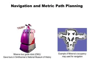
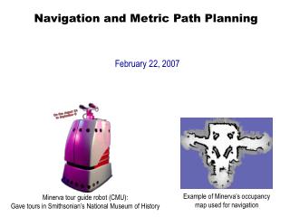
Spatial Memory • What’s the Best Way There? depends on the representation of the world • A robot’s world representation and how it is maintained over time is its spatial memory • Attention • Reasoning • Path planning • Information collection • Two forms • Route (or qualitative) • Layout (or metric) • Layout leads to Route, but not the other way Chapter 10: Metric Path Planning
Representing Area/Volume in Path Planning In Quantitative or metric maps: Rep: Many different ways to represent an area or volume of space Looks like a “bird’s eye” view, position & viewpoint independent Algorithms Graph or network algorithms Wavefront or graphics-derived algorithms Chapter 10: Metric Path Planning
Metric Maps • Motivation for having a metric map is often path planning (others include reasoning about space…) • Determine a path from one point to goal • Generally interested in “best” or “optimal” • What are measures of best/optimal? • Relevant: occupied or empty • Path planning assumes an a priori map of relevant aspects • Only as good as last time map was updated Chapter 10: Metric Path Planning
Metric Maps use Cspace • World Space: physical space robots and obstacles exist in • In order to use, generally need to know (x,y,z) plus Euler angles: 6DOF • Ex. Travel by car, what to do next depends on where you are and what direction you’re currently heading • Configuration Space (Cspace) • Is a data structure which allows the robot to specify the position (location and orientation) of any objects and the robot. • space into a representation suitable for robots, simplifying assumptions 6DOF 3DOF Chapter 10: Metric Path Planning
Major Cspace Representations • Idea: reduce physical space to a cspace representation which is more amenable for storage in computers and for rapid execution of algorithms • Major types • Meadow Maps • Generalized Voronoi Graphs (GVG) • Regular grids, quadtrees Chapter 10: Metric Path Planning
Meadow Maps • Example of the basic procedure of transforming world space to cspace • Step 1 (optional): grow obstacles as big as robot Chapter 10: Metric Path Planning
Meadow Maps cont. • Step 2: Construct convex polygons as line segments between pairs of corners, edges • Why convex polygons? Interior has no obstacles so can safely transit (“freeway”, “free space”) • Oops, not necessarily unique set of polygons Chapter 10: Metric Path Planning
Meadow Maps cont. • Step 3: represent convex polygons in way suitable for path planning-convert to a relational graph • Is this less storage, data points than a pixel-by-pixel representation? Chapter 10: Metric Path Planning
Problems with Meadow Maps • Not unique generation of polygons • Could you actually create this type of map with sensor data? • How does it tie into actually navigating the path? • How does robot recognize “right” corners, edges and go to “middle”? • What about sensor noise? Chapter 10: Metric Path Planning
Path Relaxation • Get the kinks out of the path • Can be used with any cspace representation Chapter 10: Metric Path Planning
Generalized Voronoi Graphs • Imagine a fire starting at the boundaries, creating a line where they intersect, intersections of lines are nodes • Result is a relational graph Chapter 10: Metric Path Planning
Regular Grids • Bigger than pixels, but same idea • Often on order of 4inches square • Make a relational graph by each element as a node, connecting neighbors (4-connected, 8-connected) • Moore’s law effect: fast processors, cheap hard drives, who cares about overhead anymore? Chapter 10: Metric Path Planning
Problems with GVG and Regular Grids • GVG • Sensitive to sensor noise • Path execution: requires robot to be able to sense boundaries • Grids • World doesn’t always line up on grids • Digitalization bias: left over space marked as occupied Chapter 10: Metric Path Planning
Summary of Representations • Metric path planning requires • Representation of world space, usually try to simplify to cspace • Algorithms which can operate over representation to produce best/optimal path • Representation • Usually try to end up with relational graph • Regular grids are currently most popular in practice, GVGs are interesting • Tricks of the trade • Grow obstacles to size of robot to be able to treat holonomic robots as point • Relaxation (string tightening) • Metric methods often ignore issue of • how to execute a planned path • Impact of sensor noise or uncertainty, localization Chapter 10: Metric Path Planning
Algorithms • For Path planning • A* for relational graphs • Wavefront for operating directly on regular grids • For Interleaving Path Planning and Execution Chapter 10: Metric Path Planning
Motivation for A* • Single Source Shortest Path algorithms are exhaustive, visiting all edges • Can’t we throw away paths when we see that they aren’t going to the goal, rather than follow all branches? • This means having a mechanism to “prune” branches as we go, rather than after full exploration • Algorithms which prune earlier (but correctly) are preferred over algorithms which do it later. Issue -> the mechanism for pruning Chapter 10: Metric Path Planning
A* • Similar to breadth-first: at each point in the time the planner can only “see” it’s node and 1 set of nodes “in front” • Idea is to rate the choices, choose the best one first, throw away any choices whenever you can • f*(n) is the “goodness” of the path from Start to n • g*(n) is the “cost” of going from the Start to node n • H*(n) is the cost of going from n to the Goal • H is for “heuristic function” because must have a way of guessing the cost of n to Goal since can’t see the path between n and the Goal f*(n)=g*(n)+h*(n) Chapter 10: Metric Path Planning
A* Heuristic Function • G*(n) is easy: just sum up the path costs to n • H*(n) is tricky • But path planning requires an a priori map • Metric path planning requires a METRIC a priori map • Therefore, know the distance between Initial and Goal nodes, just not the optimal way to get there • H*(n)= distance between n and Goal f*(n)=g*(n)+h*(n) Chapter 10: Metric Path Planning
Example: A to E 1 F E 1 • But since you’re starting at A and can only look 1 node ahead, this is what you see: 1.4 D 1.4 1 1 B A E D 1.4 1 B A Chapter 10: Metric Path Planning
E 1.4 2.24 D 1.4 • Two choices for n: B, D • Do both • f*(B)=1+2.24=3.24 • f*(D)=1.4+1.4=2.8 • Can’t prune, so much keep going (recurse) • Pick the most plausible path first => A-D-?-E 1 B A Chapter 10: Metric Path Planning
1 E F 1 1.4 D 1.4 1 B A • A-D-?-E • “stand on D” • Can see 2 new nodes: F, E • f*(F)=(1.4+1)+1=3.4 • f*(E)=(1.4+1.4)+0=2.8 • Three paths • A-B-?-E >= 3.24 • A-D-E = 2.8 • A-D-F-?-D >=3.4 • A-D-E is the winner! • Don’t have to look farther because expanded the shortest first, others couldn’t possibly do better without having negative distances, violations of laws of geometry… Chapter 10: Metric Path Planning
Wavefront Planners • Idea: • Considers the Cspace to be a conductive material with heat radiating out from the initial node to the goal node. • Obstacles have conductivity 0.0 • Open area infinite conductivity but undesirable terrains, which are traversable are given lower conductivity • Consider Region coloring in graphics, where color spreads out to neighboring pixels • Result: • A map which looks like a potential field Chapter 10: Metric Path Planning
Wavefront Planners Well suited for grid types of representations Chapter 10: Metric Path Planning
Trulla Chapter 10: Metric Path Planning
Interleaving Path Planning and Reactive Execution • Most Path Planning algorithms are employed in strictly plan once, then reactively execute styles. • Graph-based planners generate a path and subpaths or subsegments • Recall NHC, AuRA • Pilot looks at current subpath, instantiates behaviors to get from current location to subgoal • What happens if blocked? What happens if avoid an obstacle and actually is now closer to the next subgoal? • Causes Subgoal obsession • When does the robot think it has reached (x,y)? What about encoder error? • Need a Termination condition, usually +/- width of robot Chapter 10: Metric Path Planning
Trulla Example Chapter 10: Metric Path Planning
Two Example Approaches • If compute all possible paths in advance, not a problem • Shortest path between pairs will be part of shortest path to more distant pairs • D* • Tony Stentz • Run A* over all possible pairs of nodes • Dynamically repair A* paths affected by the changes in the map • Trulla • Ken Hughes • By-product of wave propagation style is path to everywhere Chapter 10: Metric Path Planning
Summary • Metric path planners • graph-based (A* is best known) • Wavefront • Graph-based generate paths and subgoals. • Good for NHC styles of control • In practice leads to: • Subgoal obsession • Termination conditions • Planning all possible paths helps with subgoal obsession • What happens when the map is wrong, things change, missed opportunities? How can you tell when the map is wrong or that’s it worth the computation? Chapter 10: Metric Path Planning