Download
1 / 42
450 likes | 582 Views
Path Planning Techniques . Sasi Bhushan Beera Shreeganesh Sudhindra. Path Planning. Compute motion strategies, e.g., Geometric paths Time-parameterized trajectories Achieve high-level goals, e.g., To build a collision free path from start point to the desired destination

E N D
Path Planning Techniques Sasi Bhushan Beera Shreeganesh Sudhindra
Path Planning • Compute motion strategies, e.g., • Geometric paths • Time-parameterized trajectories • Achieve high-level goals, e.g., • To build a collision free path from start point to the desired destination • Assemble/disassemble the engine • Map the environment
Objective • To Compute a collision-free path for a mobile robot among static obstacles. • Inputs required • Geometry of the robot and of obstacles • Kinematics of the robot (d.o.f) • Initial and goal robot configurations (positions & orientations) • Expected Result Continuous sequence of collision-free robot configurations connecting the initial and goal configurations
Some of the existing Methods • Visibility Graphs • Roadmap • Cell Decomposition • Potential Field
Visibility Graph Method • If there is a collision-free path between two points, then there is a polygonal path that bends only at the obstacles vertices. • A polygonal path is a piecewise linear curve.
Visibility Graph • A visibility graph is a graph such that • Nodes: qinit, qgoal, or an obstacle vertex. • Edges: An edge exists between nodes u and v if the line segment between u and v is an obstacle edge or it does not intersect the obstacles.
Breadth-First Search Slide 10
Breadth-First Search Slide 11
Breadth-First Search Slide 12
Breadth-First Search Slide 13
Breadth-First Search Slide 14
Breadth-First Search Slide 15
Breadth-First Search Slide 16
Breadth-First Search Slide 17
Breadth-First Search Slide 18
Road mapping Technique • Visibility graph • Voronoi Diagram • Introduced by computational geometry researchers. • Generate paths that maximizes clearance • Applicable mostly to 2-D configuration spaces
Cell-decomposition Methods • Exact cell decomposition • Approximate cell decomposition • F is represented by a collection of non-overlapping cells whose union is contained in F. • Cells usually have simple, regular shapes, e.g., rectangles, squares. • Facilitate hierarchical space decomposition Slide 21
Quadtree Decomposition Slide 22
Octree Decomposition Slide 23
Algorithm Outline Slide 24
Potential Fields • Initially proposed for real-time collision avoidance [Khatib 1986]. • A potential field is a scalar function over the free space. • To navigate, the robot applies a force proportional to the negated gradient of the potential field. • A navigation function is an ideal potential field that • has global minimum at the goal • has no local minima • grows to infinity near obstacles • is smooth Slide 25
Attractive & Repulsive Fields Slide 26
How Does It Work? Slide 27
Algorithm Outline • Place a regular grid G over the configuration space • Compute the potential field over G • Search G using a best-first algorithm with potential field as the heuristic function Note: A heuristic function or simply a heuristic is a function that ranks alternatives in various search algorithms at each branching step basing on an available information in order to make a decision which branch is to be followed during a search. Slide 28
Use the Local Minima Information • Identify the local minima • Build an ideal potential field – navigation function – that does not have local minima • Using the calculations done so far, we can create a PATH PLANNER which would give us the optimum path for a set of inputs. Slide 29
Active Sensing The main question to answer:”Where to move next?” Given a current knowledge about the robot state and the environment, how to select the next sensing action or sequence of actions. A vehicle is moving autonomously through an environment gathering information from sensors. The sensor data are used. to generate the robot actions Beginning from a starting configuration (xs,ys,s) to a goal configuration (xg,yg,g) in the presence of a reference trajectory and without it; With and without obstacles; Taking into account the constraints on the velocity, steering angle, the obstacles, and other constraints …
Active Sensing of a WMR Robot model
Trajectory optimization • Between two points there are an infinite number of possible trajectories. But not each trajectory from the configuration space represents a feasible trajectory for the robot. • How to move in the best way according to a criterion from the starting to a goal configuration? • The key idea is to use some parameterized family of possible trajectories and thus to reduce the infinite-dimensional problem to a finitely parametrized optimization problem. To characterize the robot motion and to process the sensor information in efficient way, an appropriate criterion is need. So, active sensing is a decision making, global optimization problem subject to constraints.
Trajectory Optimization • Let Q is a class of smooth functions. The problem of determining the ‘best’ trajectory q with respect to a criterion J can be then formulated as q = argmin(J) where the optimization criterion is chosen of the form information part losses (time, traveled distance) subject to constraints l: lateral deviation, v: WMR velocity; : steering angle; d : distance to obstacle
Trajectory Optimization The class Q of harmonic functions is chosen, Q = Q(p), p: vector of parameters obeying to preset constraints; Given N number of harmonic functions, the new modified robot trajectory is generated on the basis of the reference trajectory by a lateral deviation as a linear superposition
Why harmonic functions? • They are smooth periodic functions; • Gives the possibility to move easily the robot to the desired final point; • Easy to implement; • Multisinusoidal signals are reach excitation signals and often used in the experimental identification. They have proved advantages for control generation of nonholonomic WMR (assure smooth stabilization). For canonical chained systems Brockett (1981) showed that optimal inputs are sinusoids at integrally related frequencies, namely 2, 2. 2, …, m/2. 2.
Optimality Criterion I = trace(WP), I is computed at the goal configuration or on the the whole trajectory (part of it, e.g. in an interval ) where W = MN; M: scaling matrix; N: normalizing matrix P: estimation error covariance matrix (information matrix or entropy) from a filter (EKF);
Trajectory (N=2 sinusoids) Lyudmila Mihaylova, Katholieke Universiteit Leuven, Division PMA
Implementation • Using Optimization Toolbox of MATLAB, • fmincon finds the constrained minimum of a function of several variables • With small number of sinusoids (N<5) the computational complexity is such that it is easily implemented on-line. With more sinusoidal terms (N>10), the complexity (time, number of computations) is growing up and a powerful computer is required or off-line computation. All the performed experiments prove that the trajectories generated even with N=3 sinusoidal terms respond to the imposed requirements. Lyudmila Mihaylova, Katholieke Universiteit Leuven, Division PMA
Conclusions An effective approach for trajectories optimization has been considered : • Appropriate optimality criteria are defined. The influence of the different factors is decoupled; • The approach is applicable in the presence of and without obstacles.
Few Topics with related videos of work done by people around the world in the field Robot navigation • 3-D path planning and target trajectory prediction : http://www.youtube.com/watch?v=pr1Y21mexzs&feature=related • Path Planning : http://www.youtube.com/watch?v=d0PluQz5IuQ • Potential Function Method – By Leng Feng Lee : http://www.youtube.com/watch?v=Lf7_ve83UhE • Real-Time Scalable Motion Planning for Crowds -http://www.youtube.com/watch?v=ifimWFs5-hc&NR=1 • Robot Potential with local minimum avoidance -http://www.youtube.com/watch?v=Cr7PSr6SHTI&feature=related
References • Tracking, Motion Generation and Active Sensing of Nonholonomic Wheeled Mobile Robots -Lyudmila Mihaylova & Katholieke Universiteit Leuven • Robot Path Planning - By William RegliDepartment of Computer Science(and Departments of ECE and MEM)Drexel University • Part II-Motion Planning- by Steven M. LaValle (University of Illinois) • Wikipedia • www.mathworks.com