Download
1 / 38
380 likes | 387 Views
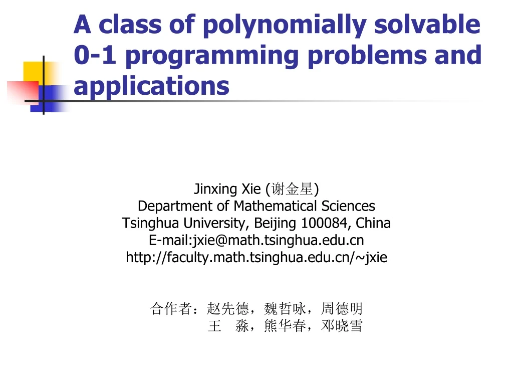
A class of polynomially solvable 0-1 programming problems and applications. Jinxing Xie ( 谢金星 ) Department of Mathematical Sciences Tsinghua University, Beijing 100084, China E-mail:jxie@math.tsinghua.edu.cn http://faculty.math.tsinghua.edu.cn/~jxie 合作者:赵先德,魏哲咏,周德明

E N D
A class of polynomially solvable 0-1 programming problems and applications Jinxing Xie (谢金星) Department of Mathematical Sciences Tsinghua University, Beijing 100084, China E-mail:jxie@math.tsinghua.edu.cn http://faculty.math.tsinghua.edu.cn/~jxie 合作者:赵先德,魏哲咏,周德明 王 淼,熊华春,邓晓雪
Outline • Background: Early Order Commitment • An Analytical Model: 0-1 Programming • A Polynomial Algorithm • Other Applications
Connect Supply With Demand: The most important issue in supply chain management (SCM) Information SUPPLY DEMAND Product Cash Supply chain optimization & coordination (SCO & SCC): The members in a supply chain cooperate with each other to reach the best performance of the entire chain
Supply Chain Coordination:Dealing with Uncertainty • Uncertainty indemand and leadtime (提前期) • Leadtime reduction: time-based competition SUPPLY DEMAND • Make to stock • Make to order
Supply Chain Coordination:Dealing with Uncertainty • Information sharing– sharing real-time demand data collected at the point-of-sales with upstream suppliers (e.g., Lee, So and Tang (LST,2000); Cachon and Fisher 2000; Raghunathan 2001; etc.) • Centralized forecasting mechanism – CPFR • Contract design – coordinate the chain • ……
Early Order Commitment (EOC) • means that a retailer commits to purchase a fixed-order quantity and delivery time from a manufacturer before the real need takes place and in advance of the leadtime. (advance ordering/booking commitment) • is used in practice for a long time, e.g. by Walmart • is an alternative form of supply chain coordination (SCC)
EOC: Questions • Why should a retailer make commitment with penalty charge? • Intuition: EOC increases a retailer’s risks of demand uncertainty, but helps the manufacturer reduce planning uncertainty • Our work • Simulation studies • Analytical model for a supply chain with infinite time horizon
EOC: Simulation Studies • Zhao, Xie and Lau (IJPR2001), Zhao, Xie and Wei (DS2002), Zhao, Xie and Zhang (SCM2002), etc. conducted extensive simulation studies under various operational conditions. • Findings • EOC can generate significant cost savings in some cases • Can we have an analytical model? (Zhao, Xie and Wei (EJOR2007), Xiong, Xie and Wang (EJOR2010), etc.)
Supplier (Manufacturer) Demand Retailer Basic Assumptions: Same asLST(MS, 2000) • The demand is assumed to be a simple autocorrelated AR(1) process • d > 0, -1<<1, and is i.i.d. normally distributed with mean zero and variance 2. • << d negative demand is negligible
Notation • L - manufacturing (supplier) leadtime • l - delivery leadtime • A - EOC period 0 <= A <= L+1 • Further (techinical) assumptions: • An “alternative” source exists for the manufacturer • Backorder for the retailer • No fixed ordering cost • Information sharing between the two partners A l Order Delivery leadtime
An order and delivery flow • PT = L, DT = l, EOCT = A (decision)
Time Label t-A t-A+1 t t+1 t+A t+l+A+1 Retailer’s Demand Dt Dt+1Dt+l+A+1 Retailer’s Order Ot-AOt-A+1 Ot Ot+L-A+1 Manufacturer’s Demand D’tD’t+1D’t+A D’t+L+1 Manufacturer’s Order Qt Time Label t t+1 t+A t+L-A+1 t+L+1 Framework of Decision Making : Periodic-review (at end of each period)
Retailer’s Ordering Decision (1) • the total demand during periods [t+1, t+l+A+1]
Retailer’s Ordering Decision (2) • the order-up-to level (optimal) • retailer’s order quantity at period t
Manufacturer’s Ordering Decision (1) • Manufacturer’s demand for [t+1, t+L+1] is
Manufacturer’s Ordering Decision (3) • The order-up-to level (optimal) • order quantity at period t is
Cost Measures • Retailer’s average cost per period • Manufacturer’s average cost per period • total cost of the supply chain Normal Loss Function
Supply Chain’s Relative Cost Saving “Cost Ratio” • Critical condition when EOC is beneficial
How ∆SC changes with A? • Theorem.∆SC decreases at first and then increases as A increases from 0 to L+1. • Corollary. The optimal A* = 0 or L+1. • Managerial implications -- Either do not use EOC policy (make to stock) or use the largest possible EOC periods (make to order)
Note on τ: usually, τ 1 Observation.(H+P)η(x)+Hxis convex in xand its minimum is achieved at K Usually: h H, p P(h+p)η(k)+hk (H+P)η(K)+HK under most situations in practice, cost ratio τ 1
How τ, l, Linfluence the performance of EOC? • Proposition 1. When τ1, EOC is always beneficial. • Proposition 2. When τ>1, as r increases, the critical condition is getting difficult to hold. • Proposition 3. When τ>1, as L increases, the critical condition is getting difficult to hold. • Proposition 4. When τ>1 and , as l increases, (LHS – RHS) of the critical condition inequality increases at first and then decreases.
EOC: Multiple retailers • i=1, 2, …, n:
EOC: 0-1 programming • i=1, 2, …, n: xi=0,or xi=L+1 • Similar to previous analysis:
EOC: 0-1 programming • Theorem
EOC: Algorithm • 算法:
EOC: generations • From 2-stage to more stages
i=1 m m-1 j ...... 1 ...... Cmi Cm-1,i Cji C1i Stage Component Base-assembly End Product Other applications • Single period problem: commonality decision in a multi-product multi-stage assembly line • For each stage j: commonality Cjc with ...... i=n
Commonality decision • Assumptions: salvage=0; stockout not permitted • Turn to spot market: the purchasing cost of the component Cji is eji (i=1,2,…,n,c ; j= m,m-1,…,1) • assume ejc ≥ eji > cji (i=1,2,…,n; j= m,m-1,…,1) • Decisions: • Whether dedicated component Cji should be replaced by the common components Cjc • Inventory levels for all components Cji (i=1,2,…,n,c ; j= m,m-1,…,1)
Commonality decision • Objective function (expected profit)
Commonality decision • Denote • Proposition. Suppose that the component commonality decision is given, then
Two different cases • Case (a) (Component commonality): • The component commonality decisions in a stage are independent of those in other stages. • Case (b) (Differentiation postponement): • The dedicated component Cji can be replaced by the common component Cjc only if the dedicated components Cj+1,i , Cj+2,i,…,Cmi are replaced by Cj+1,c , Cj+2,c ,…,Cmc (i.e., , for any and i=1,2,…,n).
Case (a) • 0-1 Programming which can be decoupled into m sub-problems (for j ) • In an optimal solution:
Case (a) • rji be the ranking position of bji among {bj1, bj2, … , bjn} O(mn2)
Case (b) • 0-1 programming • Enumeration method: • An algorithm with complexity
Other applications? • Basic patterns: square-root function + linear function • Risk management?