Download
1 / 83
830 likes | 981 Views
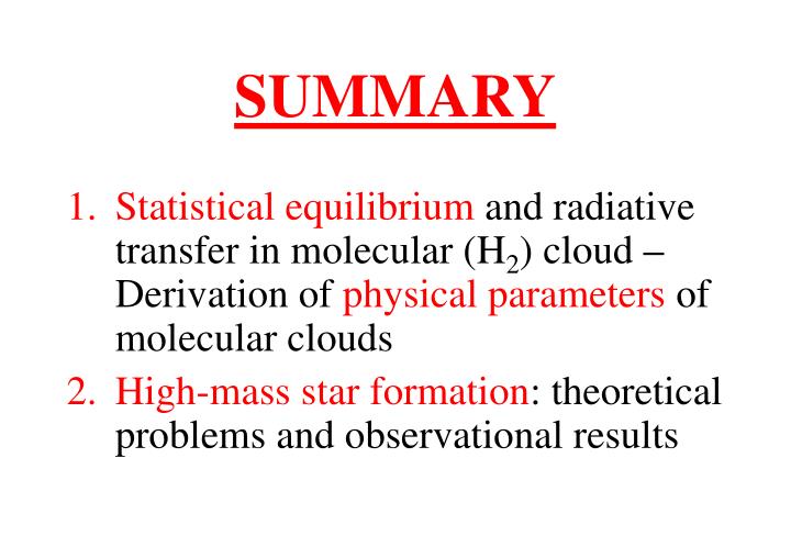
SUMMARY. Statistical equilibrium and radiative transfer in molecular (H 2 ) cloud – Derivation of physical parameters of molecular clouds High-mass star formation : theoretical problems and observational results. Statistical equilibrium and radiative transfer.

E N D
SUMMARY • Statistical equilibrium and radiative transfer in molecular (H2) cloud – Derivation of physical parameters of molecular clouds • High-mass star formation: theoretical problems and observational results
Statistical equilibriumandradiative transfer • Statistical equilibrium equations: coupling with radiation field • The excitation temperature: emission, absorption, and masers • The 2-level system: thermalization • The 3-level system: population inversion maser
Problem: Calculate molecular line brightness Iνas a function ofcloud physical parameters calculate populations ni of energy levels of given molecule X inside cloud of H2 with kinetic temperature TK and density nH2 plus external radiation field. Note:nX << nH2always; e.g. CO most abundant species but nCO/ nH2 = 10-4 !!!
… i Aij Bji Cji Bij Cij j …
2 A21 B12 C12 B21 C21 1
3-level system 3 A32 B23 C23 B32 C32 A31 B13 C13 B31 C31 2 A21 B12 C12 B21 C21 1
J=2 A21≈ 10 A10 A31 = 0 A21 J=1 A10 J=0
nH2~ ncr Tex(1-0) >TK
nH2~ ncr Tex(1-0) < 0 i.e. pop. invers. MASER!!!
Radio observations • Useful definition: brightness temperature, TB • In the radio regime Rayleigh-Jeans (hν<< kT) holds: • In practice one measures mean TB over antenna beam pattern, TMB: • Flux measured inside solid angle Ω:
Angular resolution: HPBW = 1.2 λ/D • Beam almost gaussian: ΩB = π/(4ln2)HPBW2 One measures convolution of source with beam Example gaussian source gaussian image with: • TMB = TBΩS/(ΩB+ ΩS) • Sν = (2k/λ2) TBΩS = (2k/λ2) TMB (ΩB+ ΩS) • ΘS’ = (ΘS2 + ΘB2)1/2
‘‘extended’’ source: ΩS>> ΩB TMB≈ TB ‘‘pointlike’’ source: ΩS<< ΩB TMB ≈ TB ΩS/ΩB << TB
Estimate of physical parametersof molecular clouds • Observables: TMB(orFν), ν,ΩS • Unknowns:V, TK, NX, MH2, nH2 • V velocity field • TK kinetic temperature • NX column density of molecule X • MH2 gas mass • nH2gas volume density
Velocity field From line profile: • Doppler effect: V = c(ν0- ν)/ν0 along line of sight • in most cases line FWHMthermal< FWHMobserved • thermal broadening often negligible • line profile due to turbulence & velocity field Any molecule can be used!
Star Forming Region channel maps integral under line
rotating disk line of sight to the observer
GG Tau disk 13CO(2-1) channel maps 1.4 mm continuum Guilloteau et al. (1999)
GG Tau disk 13CO(2-1) & 1.3mm cont. near IR cont.
infalling envelope line of sight to the observer
VLA channel maps 100-m spectra red-shifted absorption bulk emission blue-shifted emission Hofner et al. (1999)
Problems: • only V along line of sight • position of molecule with V is unknown along line of sight • line broadening also due to micro-turbulence • numerical modelling needed for interpretation
Kinetic temperature TKand column density NX LTEnH2>> ncr TK = Tex τ>> 1: TK≈ (ΩB/ΩS) TMB but no NX! e.g. 12CO τ<< 1: Nu (ΩB/ΩS) TMB e.g. 13CO, C18O, C17O TK= (hν/k)/ln(Nlgu/Nugl) NX = (Nu/gu) P.F.(TK) exp(Eu/kTK)
τ ≈ 1:τ = -ln[1-TMB(sat)/TMB(main)] e.g. NH3 TK= (hν/k)/ln(g2τ1/g1τ2) Nu τTK NX = (Nu/gu) P.F.(TK) exp(Eu/kTK)
If Ni is known for >2 lines TK and NX from rotation diagrams (Boltzmann plots): e.g. CH3C2H P.F.=Σ giexp(-Ei/kTK) partition function
CH3C2H Fontani et al. (2002)
CH3C2H Fontani et al. (2002)
Non-LTE numerical codes (LVG) to model TMB by varying TK, NX, nH2e.g. CH3CN Olmi et al. (1993)
Problems: • calibration error at least 10-20% on TMB • TMB is mean value over ΩB and line of sight • τ>> 1 only outer regions seen • different τ different parts of cloud seen • chemical inhomogeneities different molecules from different regions • for LVG collisional rates with H2 needed
Possible solutions: • high angular resolution small ΩB • high spectral resolution parameters of gas moving at different V’salong line profile line interferometry needed!
Mass MH2and density nH2 • Column density: MH2 (d2/X)∫ NX dΩ • uncertainty on X by factor 10-100 • error scales like distance2 • Virial theorem: MH2 d ΘS(ΔV)2 • cloud equilibrium doubtful • cloud geometry unknown • error scales like distance
(Sub)mm continuum: MH2 d2 Fν/TK • TK changes across cloud • error scales like distance2 • dust emissivity uncertain depending on environment • Non-LTE: nH2 from numerical (LVG) fit to TMB of lines of molecule far from LTE, e.g. C34S • results model dependent • dependent on other parameters (TK, X, IR field, etc.) • calibration uncertainty > 10-20% on TMB • works only for nH2≈ ncr
τ> 1 thermalization observed TB observed TB ratio TK = 20-60 K nH2≈ 3 106 cm-3 satisfy observed values
best fits to TB of four C34S lines (Olmi & Cesaroni 1999)
Bibliography • Walmsley 1988, in Galactic and Extragalactic Star Formation, proc. of NATO Advanced Study Institute, Vol. 232, p.181 • Wilson & Walmsley 1989, A&AR 1, 141 • Genzel 1991, in The Physics of Star Formation and Early Stellar Evolution, p. 155 • Churchwell et al. 1992, A&A 253, 541 • Stahler & Palla 2004, The Formation of Stars
The formation of high-mass stars: observations and problems (high-mass star M*>8M⊙ L*>103L⊙ B3-O) • Importance of high-mass stars: their impact • High- and low-mass stars: differences • High-mass stars: observational problems • The formation of high-massstars: where • The formation of high-massstars: how
Importance of high-mass stars • Bipolar outflows, stellar winds, HII regions destroy molecular clouds but may also trigger star formation • Supernovae enrich ISM with metals affect star formation • Sources of: energy, momentum, ionization, cosmic rays, neutron stars, black holes, GRBs • OB stars luminous and short lived excellent tracers of spiral arms
Stellar initial mass function (Salpeter IMF): dN/dM M-2.35N(10MO) = 10-2 N(1MO) • Stellar lifetime: t Mc2/L M-3 t(10MO) = 10-3 t(1MO) • 1051 MO stars per 10 MO star! Total mass dominated by low-mass stars. However… • Stellar luminosity: L M4 L(10MO) = 104 L(1MO)Luminosity of stars with mass between M1 and M2: • L(10-100MO) = 0.3 L(1-10MO) Luminosity of OB stars is comparable to luminosity of solar-type stars!
The formation of high-mass and low-mass stars: differences and theoretical problems
stars < 8MO isothermal unstable clump accretion onto protostar disk & outflow formation disk without accretion protoplanetary disk sub-mm far-IR near-IR visible+NIR visible
stars > 8MO isothermal unstable clump accretion onto protostar disk & outflow formation disk without accretion protoplanetary disk sub-mm far-IR near-IR visible+NIR visible ?
nR-2 nR-3/2 Low-mass VS High-mass Two mechanisms at work: Accretion onto protostar: Static envelope: nR-2 Free-falling core: nR-3/2 tacc= M*/(dMacc/dt) Contraction of protostar: tKH=GM2/R*L* • Stars < 8 Msun: tKH > tacc • Stars > 8 Msun: tKH < tacc High-mass stars form still in accretion phase