Download
1 / 28
280 likes | 375 Views
Fractal Financial Market Analysis. Seiji Armstrong Huy Luong Alon Arad Kane Hill. Outline. Seiji Introduction , History of Fractal Huy: Failure of the Gaussian hypothesis Alon: Fractal Market Analysis Kane: Evolution of Mandelbrot’s financial models.

E N D
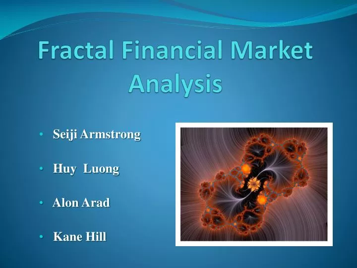
Fractal Financial Market Analysis Seiji Armstrong Huy Luong Alon Arad Kane Hill
Outline Seiji Introduction , History of Fractal Huy: Failure of the Gaussian hypothesis Alon: Fractal Market Analysis Kane: Evolution of Mandelbrot’s financial models
Fractal: Self Similarity on any scale 1x 8x Sierpinski Triangle, D = ln3/ln2 Mandelbrot Set, D = 2
Natural Fractal: Self affinity on any scale
Fractals are Everywhere: Found in Nature and Art Mathematical Formulation: Leibniz in 17th century Georg Cantor in late 19th century Mandelbrot, Godfather of Fractals: late 20th century “How long is the coastline of Britain” Latin adjective Fractus, derivation offrangere: to create irregular fragments. History: Birth of Fractal
Fractal Fern Leaf • Locally random and Globally deterministic • Underlying Stochastic Process • Similar system to financial markets !
Theory of Speculation: Louis Bachelier- 1900 Consider a time series of stock price x(t) and designate L (t,T) its natural log relative: L (t,T) = ln x(t, T) – ln x(t) where increment L(t,T) is: random statistically independent identically distributed Gaussian with zero mean Stationary Gaussian random walk
Dow Jones Index: Failure of Gaussian hypothesis
Dow Jones Index: Failure of Gaussian hypothesis
Dow Jones Index: Failure of Gaussian hypothesis
Bachelier’s Theory: Some contradictions Sample Variance of L(t,T) varies in time Tail of histogram fatter than Gaussian Large price fluctuation seen as outliers in Gaussian
Rescaled Range (R/S) Analysis Method Analyzing fractal characteristics are highly desirable for non-stationary, irregular signals. Standard methods such as Fourier are inappropriate for stock market data as it changes constantly. Fractal based methods . Relative dispersional methods , Rescaled range analysis methods do not impose this assumption
In the Beginning In 1951, Hurst defined a method to study natural phenomena such as the flow of the Nile River. Process was not random, but patterned. He defined a constant, K, which measures the bias of the fractional Brownian motion. In 1968 Mandelbrot defined this pattern as fractal. He renamed the constant K to H in honor of Hurst. The Hurst exponent gives a measure of the smoothness of a fractal object where H varies between 0 and 1.
Random and not Random It is useful to distinguish between random and non-random data points. If H equals 0.5, then the data is determined to be random. If the H value is less than 0.5, it represents anti-persistence. If the H value varies between 0.5 and 1, this represents persistence.
Calculation of R/S Start with the whole observed data set that covers a total duration and calculate its mean over the whole of the available data
Calculation of R/S Sum the differences from the mean to get the cumulative total at each time point, V(N,k), from the beginning of the period up to any time, the result is a time series which is normalized and has a mean of zero
Calculation of R/S Calculate the range
Calculation of R/S Calculate the standard deviation
Calculation of R/S Plot log-log plot that is fit Linear Regression Y on X where Y=log R/S and X=log n where the exponent H is the slope of the regression line.
Dow Jones Index: The Hurst Exponent
Fractals as a Model Gaussian market is a poor model of financial systems. A new model which will incorporate the key features of the financial market is the fractal market model.
Income Distribution (1960) Paret power law and Levy stability Long tails, skewed distributions Income categories: Skilled workers, unskilled workers, part time workers and unemployed
“Mesofractal” Model (1963) Reality: Temporal dependence of large and small price variations, fat tails Pr(U > u) ~ uα, 1 < α < 2 Infinite variance: Risk The Hurst exponent, H = ½ Brownian Motion – P(t) = BH[θ(t)]; ‘suitable subordinator’ is a stable monotone, non decreasing, random processes with independent increments Independence and fat tails : Cotton (1900-1905), Wheat price in Chicago, Railroad and some financial rates
“Unifractal” Model (1965) Fractional Brownian Motion (FBM) Brownian Motion – P(t) = BH[θ(t)] The Hurst exponent, H ≠ ½ Scale invariance – after suitable renormalization (self -affine processes are renormalizable (provide fixed points) ) under appropriate linear changes applied to t and P axes
The “Mutifractal” Model:(1972, 1997) Global property of the process’s moments Trading time is viewed as θ(t) - called the cumulative distribution function of a self similar random measure Hurst exponent is fractal variant Main differences with other models: 1. Long Memory in volatility 2. Compatibility with martingale property of returns 3. Scale consistency 4. Multi-scaling
Graphical Model comparison L1 = Brownian motion L2 = M1963 (mesofractal) L3 = M1965 (unifractal) L4 = Multifractal models L5 = IBM shares L6 = Dollar-Deutchmark exchange rate L7/8 = Multifractal models
Conclusion Neglecting the big steps More clock time - multifractal model generation.
References Mandelbrot (1960, 1961, 1962, 1963, 1965, 1967, 1972, 1974, 1997, 1999, 2000, 2001, 2003, 2005) All papers of Mandelbrot’s were used and analysed from 1960 – 2005 and can be obtained from www.math.yale.edu/mandelbrot Fractal Market Anlysis: Applying Chaos theory to Investment and Economcs(Edgar E. Peters) – John Wiley & Sons Inc. (1994)