Download
1 / 69
690 likes | 796 Views
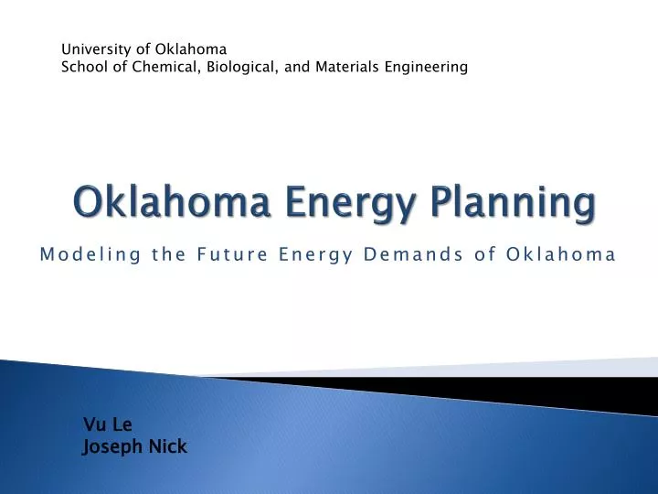
University of Oklahoma School of Chemical, Biological, and Materials Engineering. Oklahoma Energy Planning. Modeling the Future Energy Demands of Oklahoma.

E N D
University of Oklahoma School of Chemical, Biological, and Materials Engineering Oklahoma Energy Planning Modeling the Future Energy Demands of Oklahoma Vu Le Joseph Nick
So what is our project all about? Dirty EnergyClean Energy • How much will it cost energy companies? • How much will it cost Oklahoman’s? • What can the government do to foster the much needed transition?
Modeling the Future Energy Demands of Oklahoma Clean Energy Dirty Energy • Low CO2 emissions • Sustainable energy • Currently expensive • Compared to Dirty energy • High CO2 emissions • Fossil Fuel derived • CHEAP
Just how Dirty are we talking? Oklahoma’s Current Electricity Oklahoma’s Current Transportation Fuels • 52% from coal fired plants • Less than 1% from Bio-fuels Coal fired plants have the highest amount of CO2 emissions for any power plant Oklahoma total CO2 emissions from fossil fuels Over 215 billion pounds of CO2 every year!!
Objective The objective of this project is to create mathematical models that will be used to plan Oklahoma’s move toward cleaner energy through the year 2030. • Cost model - predict the optimal yearly energy use in Oklahoma, by industry, so as to minimize total energy costs (net present cost) while reducing carbon dioxide emissions and increasing total job salaries paid in Oklahoma to specified levels. • Profit model - predict the optimal yearly energy use in Oklahoma, by industry, so as to maximize total profitability, net present value. Utility pricing decisions and government tax incentives will be researched and their effect on overall profitability will be characterized.
Project goals • Develop Cost model • Develop Profit model • Model all energy used in Oklahoma from 2010 - 2030 Easy enough right??
Assumptions, Approximations, and Estimations • Forecasted U.S. natural gas consumption data – available • Forecasted Okla. natural gas consumption data – not available How accurate are forecasted commodity prices? Oil Refinery’s Revenues • Vary month to month & year to year • Vary from refinery to refinery • Each one produces different products
Assumptions • Location is not considered • Constant operation cost for plants and refineries • Switchgrass used as ethanol feedstock • Soybean used as biodiesel feedstock • Construction times for new plants • Wind – 1 year • Everything else – 3 years
Energy Types Electricity • Coal-fired plants • Natural gas fired plants • Hydroelectric plants • Wind farms Fuels • Gasoline and Diesel • Biodiesel • Ethanol Heating • Residential • Commercial • Industrial • Plant
Research • Past • data • Present • data • Projected • data • Energy Information Administration • U.S. Department of Energy • Oklahoma Wind Power Initiative • Oklahoma Renewable Energy Council • Some forecasted data was readily available, while other data had to be independently forecasted by us.
Research Examples of required data in calculating: • Total cost of energy • Total carbon dioxide emissions • Total Revenues • Total salaries paid to Oklahoma workers • Number of existing plants (by type) • Capacity of existing plants • Total plant operating hours • Plant CO2 emissions • Current fuel prices • Forecasted fuel prices • Forecasted energy demand (by type) • Forecasted energy supply (by type) • Cost of building new plants
Electricity • Coal and natural gas plants • Hydroelectric plants and Wind farms Fig.1 A coal fired power plant Fig.2 Repower wind turbines Fig. 3 A hydroelectric Dam
Transportation Fuels • Gasoline and Diesel • (Crude Oil Refineries) • Biodiesel and Ethanol Refineries Sunflower field, Biodiesel production Switch grass field, Ethanol production Canadian Sand Oil Field
Ethanol Cellulosic biomass (switchgrass) processing cellulose enzymatic breakdown & pyrolysis sugars fermentation ETHANOL Fig. The CO2 cycle of ethanol production
Heating • Electricity • Natural Gas (Clockwise from bottom left) Residential-Household use Industrial- Heat, power, and chemical feedstock use Commercial-Use by non-manufacturing establishments Plant-Fuel use in N.G. processing plants
Natural Gas • Various estimates place natural gas at 75-90% of total heating (all sectors)
Cost Model Operation Total Cost ‘i’ = (Fixed Opr. Cost) + (Var. Opr. Cost) + (Fuel Cost) + (Capital Cost) + (Expansion Cost) + (Transportation Cost) + (E Carbon Capture Cost) [(Fixed Opr. Cost) + (Var. Opr. Cost) + (Fuel Cost) + (N Carbon Capture Cost New)]new • Fuels • Heating • Electricity
Cost Model Operation Each energy type has varying data for: • Fuel cost • New plant capital cost • CO2 emissions • Existing capacity • Future demand • Job salaries creation Increased demand New plants Lower CO2 emissions Energy types with lower emissions or Carbon capture More job salaries Choose energy with most jobs Minimize Cost Choose most cost effective energy
Operating Costs Fixed operating and maintenance (Fixed O&M) costs • Salaries • Wind farm lease payments • Insurance payments Variable operating and maintenance (Var. O&M) costs • Raw material costs • Utility payments Fuel costs Electricity Coal, Natural Gas Fuels Crude Oil, Switchgrass, Soybean For both fuels and electricity, these costs were approximated as: Cost = X ∙ Capacity -or- Cost = X ∙ Fuel Used Where X is a function of the energy type.
Fixed Operating Cost The Fixed and Variable O&M costs for all 9 energy types were not readily available from one source. • Documented, credible sources. Examples of organization and company websites were used to locate our O&M cost data • Energy Information Administration • U.S. Department of Agriculture • American Wind Energy Association • Energy and Environmental Economies Incorporated • Baker & O’Brien Incorporated • Resource Dynamic Corporation
Capital Cost Capital costs are the costs of building new plants or expanding existing plants. Cost = ( X ∙ Capacity ) + Y • Unlike fixed and variable O&M costs, capital costs have a minimum associated cost and thus can not be approximated as easily. What to do? • Analyze data from previous plant constructions and plant expansions
Electricity Capital Cost • Data we were able to find made no distinctions between electricity plant fuel sources (coal, natural gas, etc) • Not including hydro-electric and wind energy • Unlike fuels, new electricity plants can be built and are not limited to expansions Minimum cost for new coal and NG plant construction, regardless of capacity ~ 259 million
Wind Capital Cost • There is no minimum installed capital cost for new wind energy operations • Capital cost is a function of capacity Cost = X ∙ capacity where X is the average installed cost per MW $ MW Installed cost = 1,750,000
Job Salary Creation We are evaluating job creation in the state of Oklahoma using total wages paid to Oklahoma workers yearly Total Salary = Existing Salaries (2009) + New Salaries New Salaries = New Operation Salaries + New Construction Salaries Operation Salaries = Wages paid to engineers and employees who work to operate and maintain energy creation facilities Example: Plant managers, plant engineers, plant operators, etc Construction Salaries = Wages paid to engineers and employees who work in constructing new energy creation facilities Example: Construction engineers, construction workers, transportation drivers
Construction Salary From Perry’s Chemical Engineers’ Handbook
New Operation Salary The following graph was constructed using data from DESIGN, figure 6-9 [1] Convert our capacity data into kg / day [2] Estimate the number of process steps involved [3] Calculate salary paid from employee hours per day required • Calculate average refinery employee’s salary • Engineers vs. non-engineer workers
Profit Model Operation Each energy type has varying data for: • New plant capital cost • Operation Costs • CCS cost • Profitability • Revenues • Explored different scenarios for: • Tax breaks • New sustainable energy types • Carbon Capture, existing plants • Job creation • Emissions and job creation • Fuels • Heating • Electricity • Minimum price to consumers to meet • specified return on investment
Algebraic Model • Indices • t time period (yrs) • i Individual boiler or refinery • j Fuel type (i.e. coal/natural gas) • Sets • newNew plants or refineries • Electric, Fuel, Heat
Algebraic Model (Profit) *only new and electric plants are shown
Model Constraints • Energy Generated must equal Demand
Model Constraints • Net CO2 Emission must be reduced by a preset limit
Model Constraints • Energy Generated must be less than capacity
Model Constraints • Job Creation in Salary must increase by a preset limit
Model Constraints • Annual profits from new plants and refineries must exceed a set ROI.
GAMS Code Model • Operation Cost • Electricity Industry • Transportation Fuel • Natural Gas Heating • CO2 Reduction • Job Salary • Profitability • 3200 Lines of Codes • ~ 2 min to run
GAMS Code (Profitability) GAMS Code (Fuel Model) GAMS Code (Fuel Model)
This surface represent the maximum NPV possible at a certain CO2 limit and Job creation for all industries combined. Pareto-optimal Boundary
Job salary creation has a minor effect on NPV • CO2 reduction has a major effect on NPV • After 2% CO2 reduction, more carbon capture technology is used. • - Primary reason for the steeper slope Pareto-optimal Boundary
Minimum Retail Electricity Price *Jobs at 1%
Minimum Retail Electricity Price *Jobs at 1% • This table shows the minimum average electricity price _require to make a profit. • Investors will not invests in new plants with no tax break
Scenarios • 4 Scenario will be presented: • Retail Price of Electricity at 10 cent/KWH • ROI at 10%