Download
1 / 39
390 likes | 549 Views
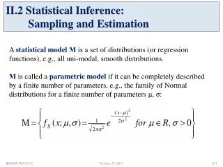
Sampling and estimation 2. Tron Anders Moger 27.09.2006. Confidence intervals (rep.). Assume that X 1 ,..,X n are a random sample from a normal distribution Recall that has expected value and variance 2 /n The interval + 1.96 / √ n is called a 95% confidence interval for

E N D
Sampling and estimation 2 Tron Anders Moger 27.09.2006
Confidence intervals (rep.) • Assume that X1 ,..,Xn are a random sample from a normal distribution • Recall that has expected value and variance 2/n • The interval + 1.96/√n is called a 95% confidence interval for • Means that the interval will contain the population mean 95% of the time • Often interpreted as if we are 95% certain that the population mean lies in this interval
Hypothesis testing (rep.) • Have a data sample • Would like to test if there is evidence that a parameter value calculated from the data is different from the value in a null hypothesis H0 • If so, means that H0 is rejected in favour of some alternative H1 • Have to construct a test statistic • It must: • Have a higher probability for ”extreme” values under H1 than under H0 • Have a known distribution under H0 (when simple)
Two important quantities • P-value = probability of the observed value or something more extreme assuming null hypothesis • Significance level α= the value at which we reject H0 • If the value of the test statistic is ”too extreme”, then H0 is rejected • P-value=0.05: We want the probability that the observed difference is due to chance to be below 5%, or, equivalently: • We want to be 95% sure that we do not reject H0when it is true in reality
Note: • There is an asymmetry between H0 and H1: In fact, if the data is inconclusive, we end up not rejecting H0. • If H0 is true the probability to reject H0 is (say) 5%. That DOES NOT MEAN we are 95% certain that H0 is true! • How much evidence we have for choosing H1 over H0 depends entirely on how much more probable rejection is if H1 is true.
Errors of types I and II • The above can be seen as a decision rule for H0 or H1. • For any such rule we can compute (if both H0 and H1 are simple hypotheses): Power 1 - β 1-α H0 true H1 true Accept H0 TYPE II error Reject H0 TYPE I error β Significance level α
Sample size computations • For a sample from a normal population with known variance, the size of the conficence interval for the mean depends only on the sample size. • So we can compute the necessary sample size to match a required accuracy • Note: If the variance is unknown, it must somehow be estimated on beforehand to do the computation • Works also for population proportion estimation, giving an inequality for the required sample size
Power computations • If you reject H0, you know very little about the evidence for H1 versus H0 unless you study the power of the test. • The power is 1 minus the probability of rejecting H0 given that a hypothesis in H1 is true (1-β). • Thus it is a function of the possible hypotheses in H1. • We would like our tests to have as high power as possible.
Example 1: Normal distribution with unknown variance • Assume • Then • Thus • So a confidence interval for , with significance is given by
Example 1 (Hypothesis testing) • Hypotheses: • Test statistic under H0 • Reject H0 if or if • Alternatively, the p-value for the test can be computed (if ) as the such that
Example 1 (cont.) • Hypotheses: • Test statistic assuming • Reject H0 if • Alternatively, the p-value for the test can be computed as the such that
Energy intake in kJ • SUBJECT INTAKE 1 5260 2 5470 3 5640 4 6180 5 6390 6 6515 7 6805 8 7515 9 7515 10 8230 11 8770 Recommended energy intake: 7725kJ Want to test if it applies to the 11 women H0: (mean energy intake)=7725 H1: 7725
Test result: • This quantity is t-distributed with 10 degrees of freedom (number of subjects -1) • Choose significance level α=0.05 • From table 8 p.870 in the book, t11-1,0.05/2=2.262 • If the H0 is true, the interval (-2.262, 2.262) covers 95% of the distribution • Reject H0 since the test statistic is outside the interval, or, equivalently, because • Can’t find exact p-value from the table • Could have had α=0.01 or 0.1, but 0.05 is most common
In SPSS: Analyze - Compare means - One-sample t testTest variable: intakeTest value: 7725
Differences between means • Assume and , all data independent • We would like to study the difference x-y • Three different cases: • Matched pairs • Unknown but equal population variances • Unknown and possibly different pop. variances
Matched pairs • Common situation: Several measurements on each individual, or on closely related objects • These measurements will not be independent (why?) • Generally a problem in statistics, but simple if you only have two measurements • The key is to use the difference between the means, instead of each mean seperately
Example 2: Matched pairs • In practice, the basis is that x-y=0 • Set and • We get • Where • Confidence interval for x-y
Example 2 (Hypothesis testing) • Hypotheses: • Test statistic: • Reject H0 if or if ”Matched pairs T test”
Example: Energy intake kJ SUBJECT PREMENST POSTMENS 1 5260.0 3910.0 2 5470.0 4220.0 3 5640.0 3885.0 4 6180.0 5160.0 5 6390.0 5645.0 6 6515.0 4680.0 7 6805.0 5265.0 8 7515.0 5975.0 9 7515.0 6790.0 10 8230.0 6900.0 11 8770.0 7335.0 Number of cases read: 11 Number of cases listed: 11 Want to test if energy intake is different before and after menstruation. H0: premenst= postmenst H1: premenst postmenst
Confidence interval and p-values for paired t-tests in SPSS • Analyze - Compare Means -Paired-Samples T Test. • Click on the two variabels you want to test, and move them to Paired variables • Conclusion: Reject H0 on 5% sig. level
Example 3: Unknown but equal population variances • We get where • Confidence interval for
Example 3 (Hypothesis testing) • Hypotheses: • Test statistic: • Reject H0 if or if ”T test with equal variances”
Assumptions • Independence: All observations are independent. Achieved by taking random samples of individuals; for paired t-test independence is achieved by using the difference between measurements • Normally distributed data (Check: histograms, tests for normal distribution, Q-Q plots) • Equal variance or standard deviations in the groups • Assumptions can be checked in histograms, box plots etc. (or tests for normality) • What if the variances are unequal?
Example 4: Unknown and possibly unequal population variances • We get where • Conf. interval for
Example 4 (Hypothesis testing) • Hypotheses: • Test statistic • Reject H0 if or if ”T test with unequal variances”
Example 5: The variance of a normal distribution • Assume • Then • Thus • Confidence interval for
Example 5: Comparing variances for normal distributions • Assume • We get • Fnx-1,ny-1 is an F distribution with nx-1 and ny-1 degrees of freedom • We can use this exactly as before to obtain a confidence interval for and for testing for example if • Note: The assumption of normality is crucial!
ID GROUP ENERGY 1 0 6.13 2 0 7.05 .... 12 0 10.15 13 0 10.88 14 1 8.79 15 1 9.19 .... 21 1 11.85 22 1 12.79 Number of cases read: 22 Number of cases listed: 22 Example: Energy expenditure in two groups, lean and obese. Want to test if there is any difference. H0: lean= obese H1: lean obese
In SPSS: • Analyze - Compare Means - Independent-Samples T Test • Move Energy to “Test-variable” • Move Group to “Grouping variable”Click “Define Groups” and write 0 and 1 for the two groups
Output: Above 0.05: Read first line (Equal variances assumed) Otherwise: Read second line (Equal variances not assumed)
Conclusion • The observed mean for the lean was 8.1, and for the obese 10.3 (mean difference -2.2, 95% confidence interval for the difference (-3.4, -1.1)) • The difference between the groups was significant on a 5%-level (since the CI does not include the value 0) • The p-value was 0.001. • H0 is rejected
Example 6: Population proportions • Assume , so that is a frequency. • Then • Thus • Thus • Confidence interval for P (approximately, for large n) (approximately, for large n)
Example 6 (Hypothesis testing) • Hypotheses: H0:P=P0 H1:PP0 • Test statistic under H0, for large n • Reject H0 if or if
Example 7: Differences between population proportions • Assume and , so that and are frequencies • Then • Confidence interval for P1-P2 (approximately)
Example 7 (Hypothesis testing) • Hypotheses: H0:P1=P2 H1:P1P2 • Test statistic where • Reject H0 if
Spontanous abortions among nurses helping with operations and other nurses • Want to test if there is difference between the proportions of abortions in the two groups • H0: Pop.nurses=Pothers H1: Pop.nursesPothers
Calculation: • P1=0.278 P2=0.088 n1=36 n2=34 z= • P-value 0.0414=4.1%, reject H0 on 5%-sig.level (can’t do this in SPSS) • 95% confidence interval for P1-P2:
Next week: • Next lecture will be about modelling relationships between continuous variables • Linear regression