Download
1 / 51
510 likes | 526 Views
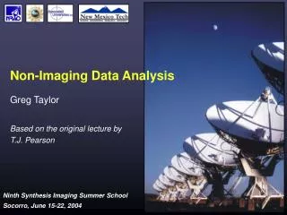
Non-Imaging Data Analysis. Greg Taylor University of New Mexico June, 2008. Outline. Introduction Inspecting visibility data Model fitting Some applications Superluminal motion Gamma-ray bursts Gravitational lenses Binary stars The Sunyaev-Zeldovich effect. Introduction.

E N D
Non-Imaging DataAnalysis • Greg Taylor • University of New Mexico • June, 2008
Outline • Introduction • Inspecting visibility data • Model fitting • Some applications • Superluminal motion • Gamma-ray bursts • Gravitational lenses • Binary stars • The Sunyaev-Zeldovich effect
Introduction • Reasons for analyzing visibility data • Insufficient (u,v)-plane coverage to make an image • Inadequate calibration • Quantitative analysis • Direct comparison of two data sets • Error estimation • Usually, visibility measurements are independent gaussian variates • Systematic errors are usually localized in the (u,v) plane • Statistical estimation of source parameters
Inspecting Visibility Data • Fourier imaging • Problems with direct inversion • Sampling • Poor (u,v) coverage • Missing data • e.g., no phases (speckle imaging) • Calibration • Closure quantities are independent of calibration • Non-Fourier imaging • e.g., wide-field imaging; time-variable sources (SS433) • Noise • Noise is uncorrelated in the (u,v) plane but correlated in the image
Useful displays Sampling of the (u,v) plane Amplitude and phase vs. radius in the (u,v) plane Amplitude and phase vs. time on each baseline Amplitude variation across the (u,v) plane Projection onto a particular orientation in the (u,v) plane Example: 2021+614 GHz-peaked spectrum radio galaxy at z=0.23 A VLBI dataset with 11 antennas from 1987 VLBA only in 2000 Inspecting Visibility Data
Properties of the Fourier transform • See, e.g., R. Bracewell, The Fourier Transform and its Applications (1965). • Fourier Transform theorems • Linearity • Visibilities of components add (complex) • Convolution • Shift • Shifting the source creates a phase gradient across the (u,v) plane • Similarity • Larger sources have more compact transforms
Simple models • Visibility at short baselines contains little • information about the profile of the source.
Trial model • By inspection, we can derive a simple model: • Two equal components, each 1.25 Jy, separated by about 6.8 milliarcsec in p.a. 33º, each about 0.8 milliarcsec in diameter (Gaussian FWHM) • To be refined later…
Closure Phase and Amplitude: closure quantities • Antenna-based gain errors • Closure phase (bispectrum phase) • Closure amplitude • Closure phase and closure amplitude are unaffected by antenna gain errors • They are conserved during self-calibration • Contain (N–2)/N of phase, (N–3)/(N–1) of amplitude info • Many non-independent quantities • They do not have gaussian errors • No absolute position or flux info l m k n
Model fitting • Imaging as an Inverse Problem • In synthesis imaging, we can solve the forward problem: given a sky brightness distribution, and knowing the characteristics of the instrument, we can predict the measurements (visibilities), within the limitations imposed by the noise. • The inverse problem is much harder, given limited data and noise: the solution is rarely unique. • A general approach to inverse problems is model fitting. See, e.g., Press et al., Numerical Recipes. • Design a model defined by a number of adjustable parameters. • Solve the forward problem to predict the measurements. • Choose a figure-of-merit function, e.g., rms deviation between model predictions and measurements. • Adjust the parameters to minimize the merit function. • Goals: • Best-fit values for the parameters. • A measure of the goodness-of-fit of the optimized model. • Estimates of the uncertainty of the best-fit parameters.
Model fitting • Maximum Likelihood and Least Squares • The model: • The likelihood of the model (if noise is gaussian): • Maximizing the likelihood is equivalent to minimizing chi-square (for gaussian errors): • Follows chi-square distribution with N – M degrees of freedom. Reduced chi-square has expected value 1.
Uses of model fitting • Model fitting is most useful when the brightness distribution is simple. • Checking amplitude calibration • Starting point for self-calibration • Estimating parameters of the model (with error estimates) • In conjunction with CLEAN or MEM • In astrometry and geodesy • Programs • AIPS UVFIT • Difmap (Martin Shepherd)
Parameters • Example • Component position: (x,y) or polar coordinates • Flux density • Angular size (e.g., FWHM) • Axial ratio and orientation (position angle) • For a non-circular component • 6 parameters per component, plus a “shape” • This is a conventional choice: other choices of parameters may be better! • (Wavelets; shapelets* [Hermite functions]) • * Chang & Refregier 2002, ApJ, 570, 447
Practical model fitting: 2021 • ! Flux (Jy) Radius (mas) Theta (deg) Major (mas) Axial ratio Phi (deg) T • 1.15566 4.99484 32.9118 0.867594 0.803463 54.4823 1 • 1.16520 1.79539 -147.037 0.825078 0.742822 45.2283 1
Model fitting 2021 • ! Flux (Jy) Radius (mas) Theta (deg) Major (mas) Axial ratio Phi (deg) T • 1.10808 5.01177 32.9772 0.871643 0.790796 60.4327 1 • 0.823118 1.80865 -146.615 0.589278 0.585766 53.1916 1 • 0.131209 7.62679 43.3576 0.741253 0.933106 -82.4635 1 • 0.419373 1.18399 -160.136 1.62101 0.951732 84.9951 1
Limitations of least squares • Assumptions that may be violated • The model is a good representation of the data • Check the fit • The errors are Gaussian • True for real and imaginary parts of visibility • Not true for amplitudes and phases (except at high SNR) • The variance of the errors is known • Estimate from Tsys, rms, etc. • There are no systematic errors • Calibration errors, baseline offsets, etc. must be removed before or during fitting • The errors are uncorrelated • Not true for closure quantities • Can be handled with full covariance matrix
Least-squares algorithms • At the minimum, the derivatives • of chi-square with respect to the • parameters are zero • Linear case: matrix inversion. • Exhaustive search: prohibitive with • many parameters (~ 10M) • Grid search: adjust each parameter by a • small increment and step down hill in search for minimum. • Gradient search: follow downward gradient toward minimum, using numerical or analytic derivatives. Adjust step size according to second derivative • For details, see Numerical Recipes.
Problems with least squares • Global versus local minimum • Slow convergence: poorly constrained model • Do not allow poorly-constrained parameters to vary • Constraints and prior information • Boundaries in parameter space • Transformation of variables • Choosing the right number of parameters: does adding a parameter significantly improve the fit? • Likelihood ratio or F test: use caution • Protassov et al. 2002, ApJ, 571, 545 • Monte Carlo methods
Error estimation • Find a region of the M-dimensional parameter space around the best fit point in which there is, say, a 68% or 95% chance that the true parameter values lie. • Constant chi-square boundary: select the region in which • The appropriate contour depends on the required confidence level and the number of parameters estimated. • Monte Carlo methods (simulated or mock data): relatively easy with fast computers • Some parameters are strongly correlated, e.g., flux density and size of a gaussian component with limited (u,v) coverage. • Confidence intervals for a single parameter must take into account variations in the other parameters (“marginalization”).
Mapping the likelihood • Press et al., • Numerical • Recipes
Applications: Superluminal motion • Problem: to detect changes in component positions between observations and measure their speeds • Direct comparison of images is bad: different (u,v) coverage, uncertain calibration, insufficient resolution • Visibility analysis is a good method of detecting and measuring changes in a source: allows “controlled super-resolution” • Calibration uncertainty can be avoided by looking at the closure quantities: have they changed? • Problem of differing (u,v) coverage: compare the same (u,v) points whenever possible • Model fitting as an interpolation method
Superluminal motion • Example 1: Discovery of superluminal motion in 3C279 (Whitney et al., Science, 1971)
Superluminal motion • 1.55 ± 0.3 milliarcsec in 4 months: v/c = 10 ± 3
3C279 with the VLBA • Wehrle et al. 2001, ApJS, 133, 297
Demo • Switch to Difmap and demo model-fiting on VLBA data
Applications: Expanding sources • Example 2: changes in the radio galaxy 2021+614 between 1987 and 2000 • We find a change of 200 microarcsec so v/c = 0.18 • By careful combination of model-fitting and self-calibration, Conway et al. (1994) determined that the separation had changed by 69 ± 10 microarcsec between 1982 and 1987, for v/c = 0.19
Applications - GRB030329 June 20, 2003 t+83 days Peak ~ 3 mJy Size 0.172 +/- 0.043 mas 0.5 +/- 0.1 pc average velocity = 3c Taylor et al. 2004 VLBA+Y27+GBT+EB+AR+WB = 0.11 km2
GRB 030329 Expansion over 3 years Apparent velocity ranging from 8c at 25 days to 1.2c after 800 days
Applications: A Binary Star • Binary Stars • Many stars are in binary systems • Orbital parameters can be used to measure stellar masses • Astrometry can provide direct distances via parallax and proper motions. • Application of model fitting • Optical interferometry provides sparse visibility coverage • Small number of components • Need error estimates. • Example: NPOI observations of Phi Herculis (Zavala et al. 2006) • Multiple observations map out the orbit
Applications: Gravitational Lenses • Gravitational Lenses • Single source, multiple images formed by intervening galaxy. • Can be used to map mass distribution in lens. • Can be used to measure distance of lens and H0: need redshift of lens and background source, model of mass distribution, and a time delay. • Application of model fitting • Lens monitoring to measure flux densities of components as a function of time. • Small number of components, usually point sources. • Need error estimates. • Example: VLA monitoring of B1608+656 (Fassnacht et al. 1999, ApJ) • VLA configuration changes: different HA on each day • Other sources in the field
1608 monitoring results • B – A = 31 days • B – C = 36 days • H0 = 75 ± 7 km/s/Mpc Koopmans et al. 2003
Applications: Sunyaev-Zeldovich effect • The Sunyaev-Zeldovich effect • Photons of the CMB are scattered to higher frequencies by hot electrons in galaxy clusters, causing a brightness decrement. • Decrement is proportional to integral of electron pressure through the cluster, or electron density if cluster is isothermal. • Electron density and temperature can be estimated from X-ray observations, so the linear scale of the cluster is determined. • This can be used to measure the cluster distance and H0. • Application of model fitting • The profile of the decrement can be estimated from X-ray observations (beta model). • The Fourier transform of this profile increases exponentially as the interferometer baseline decreases. • The central decrement in a synthesis image is thus highly dependent on the (u,v) coverage. • Model fitting is the best way to estimate the true central decrement.
SZ images Reese et al. 2002
Summary For simple sources observed with high SNR, much can be learned about the source (and observational errors) by inspection of the visibilities. Even if the data cannot be calibrated, the closure quantities are good observables, and modelfiting can help to interpret them. Quantitative data analysis is best regarded as an exercise in statistical inference, for which the maximum likelihood method is a general approach. For gaussian errors, the ML method is the method of least squares. Visibility data (usually) have uncorrelated gaussian errors, so analysis is most straightforward in the (u,v) plane. Consider visibility analysis when you want a quantitative answer (with error estimates) to a simple question about a source. Visibility analysis is inappropriate for large problems (many data points, many parameters, correlated errors); standard imaging methods can be much faster.