Download
1 / 8
80 likes | 83 Views
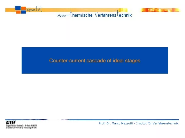
Counter-current cascade of ideal stages. Prof. Dr. Marco Mazzotti - Institut für Verfahrenstechnik. L, x 0. y 1. 3. 2. 1. y 2. x 1. y 3. x 2. G, y 4. x 3. Let’s consider three ideal stages.

E N D
Counter-current cascade of ideal stages Prof. Dr. Marco Mazzotti - Institut für Verfahrenstechnik
L, x0 y1 3 2 1 y2 x1 y3 x2 G, y4 x3 Let’s consider three ideal stages. The solvent stream enters the cascade by the first stage. The solvent can be pure or can have a certain concentration of solute, represented by xo. The gas enters the cascade by the last stage and thus, flows in counter-current to the solvent flow. The operating line is defined by points of compositions of gas and liquid phases at the same level of the process. Points on the operating line are: Because the stages are ideal, the equilibrium is reached in each of them. This means that the gas and the liquid phase going out from a stage are at equilibrium, and thus lie on the equilibrium line.
y1 L, x0 2 n j 1 dotted area solute yj yj+1 y2 x1 xj xn xj-1 G, yn+1 Mass balances Localpartial mass balance The equilibrium equation: Dividing by G: The operating line is: The slope of the operating line is positive (L/G)
y1 L, x0 j 1 2 n y y2 yj yj+1 xn x1 xj Yn+1 y = m x xj-1 x0 x G, yn+1 Data are the initial gas composition, yn+1, as well as the initial solvent composition, xo. On the diagram: When the final gas composition, y1, is known because it is restricted to be less than a certain minimum value (specification), the first point of the operating line can be set. Y1
y1 L, x0 1 2 j n y yj+1 y2 yj xn x1 xj Yn+1 L/G y = m x xj-1 x0 x G, yn+1 For the specific slope (L/G), we can set the operating line: Y1
y1 L, x0 1 2 j n y y2 yj yj+1 x1 xj xn Yn+1 y = m x xj-1 x0 x Y1 G, yn+1 The graphical resolution consists on a step by step construction. We know that x1 is at equilibrium with y1. It is then easy to set x1on the diagram. We also know that x1 and y2 are the same point on the operating line, since they are both at the same level in the cascade. And so on, until the specification is reached... Y4 Y3 Y2 x1 x2 x3 x4
A sequential resolution is also possible without the graphical representation, alternating the use of the operating line equation and the equilibrium equation. As we have seen in the case of the cross-current cascade, a mathematical resolution can also be done. Introducing the absorption factor in the mass balance equation obtained before... Comparing this equation and the general Difference Partial equation, we get And applying the general solution we get And for the n stage:
The fractional absorption can now be calculated, by substituting the value of yn+1: This is the Kremser equation. And solving for n, the number of stages can be calculated: When A=1, the Kremser equation cannot be used. The fraction of absorption is then calculated: