Download

1 / 49
490 likes | 629 Views
Statistical Debugging. Ben Liblit, University of Wisconsin–Madison. . €. ƒ. ‚. ƒ. €. . Bug Isolation Architecture. Predicates. Shipping Application. Program Source. Sampler. Compiler. Statistical Debugging. Counts & J / L. Top bugs with likely causes.

E N D
Statistical Debugging Ben Liblit, University of Wisconsin–Madison
€ ƒ ‚ ƒ € Bug Isolation Architecture Predicates ShippingApplication ProgramSource Sampler Compiler StatisticalDebugging Counts& J/L Top bugs withlikely causes
Winnowing Down the Culprits • 1710 counters • 3 × 570 call sites • 1569 zero on all runs • 141 remain • 139 nonzero on at least one successful run • Not much left! • file_exists() > 0 • xreadline() == 0
Multiple, Non-Deterministic Bugs • Strict process of elimination won’t work • Can’t assume program will crash when it should • No single common characteristic of all failures • Look for general correlation, not perfect prediction • Warning! Statistics ahead!
Ranked Predicate Selection • Consider each predicate P one at a time • Include inferred predicates (e.g. ≤, ≠, ≥) • How likely is failure when P is true? • (technically, when P is observed to be true) • Multiple bugs yield multiple bad predicates
Are We Done? Not Exactly! if (f == NULL) { x = 0; *f;} Bad(f = NULL) = 1.0
Are We Done? Not Exactly! if (f == NULL) { x = 0; *f;} Bad(f = NULL) = 1.0 Bad(x = 0) = 1.0 • Predicate (x = 0) is innocent bystander • Program is already doomed
Fun With Multi-Valued Logic • Identify unlucky sites on the doomed path • Background risk of failure for reaching this site, regardless of predicate truth/falsehood
Isolate the Predictive Value of P Does P being true increase the chance of failure over the background rate? • Formal correspondence to likelihood ratio testing
Increase Isolates the Predictor if (f == NULL) { x = 0; *f;} Increase(f = NULL) = 1.0 Increase(x = 0) = 0.0
It Works! …for programs with just one bug. • Need to deal with multiple bugs • How many? Nobody knows! • Redundant predictors remain a major problem Goal: isolate a single “best” predictor for each bug, with no prior knowledge of the number of bugs.
Multiple Bugs: Some Issues • A bug may have many redundant predictors • Only need one, provided it is a good one • Bugs occur on vastly different scales • Predictors for common bugs may dominate, hiding predictors of less common problems
Guide to Visualization • Multiple interesting & useful predicate metrics • Simple visualization may help reveal trends Increase(P) error bound Context(P) S(P) log(F(P) + S(P))
Confidence Interval on Increase(P) • Strictly speaking, this is slightly bogus • Bad(P) and Context(P) are not independent • Correct confidence interval would be larger
Bad Idea #1: Rank by Increase(P) • High Increasebut very few failing runs • These are all sub-bug predictors • Each covers one special case of a larger bug • Redundancy is clearly a problem
Bad Idea #2: Rank by F(P) • Many failing runs but low Increase • Tend to be super-bug predictors • Each covers several bugs, plus lots of junk
A Helpful Analogy • In the language of information retrieval • Increase(P) has high precision, low recall • F(P) has high recall, low precision • Standard solution: • Take the harmonic mean of both • Rewards high scores in both dimensions
Rank by Harmonic Mean • Definite improvement • Large increase, many failures, few or no successes • But redundancy is still a problem
Redundancy Elimination • One predictor for a bug is interesting • Additional predictors are a distraction • Want to explain each failure once • Similar to minimum set-cover problem • Cover all failed runs with subset of predicates • Greedy selection using harmonic ranking
Simulated Iterative Bug Fixing • Rank all predicates under consideration • Select the top-ranked predicate P • Add P to bug predictor list • Discard P and all runs where P was true • Simulates fixing the bug predicted by P • Reduces rank of similar predicates • Repeat until out of failures or predicates
Case Study: Moss • Reintroduce nine historic Moss bugs • High- and low-level errors • Includes wrong-output bugs • Instrument with everything we’ve got • Branches, returns, variable value pairs, the works • 32,000 randomized runs at 1/100 sampling
Effectiveness of Ranking • Five bugs: captured by branches, returns • Short lists, easy to scan • Can stop early if Bad drops down • Two bugs: captured by value-pairs • Much redundancy • Two bugs: never cause a failure • No failure, no problem • One surprise bug, revealed by returns!
Analysis of exif • 3 bug predictors from 156,476 initial predicates • Each predicate identifies a distinct crashing bug • All bugs found quickly using analysis results
Analysis of Rhythmbox • 15 bug predictors from 857,384 initial predicates • Found and fixed several crashing bugs
Other Models, Briefly Considered • Regularized logistic regression • S-shaped curve fitting • Bipartite graphs trained with iterative voting • Predicates vote for runs • Runs assign credibility to predicates • Predicates as random distribution pairs • Find predicates whose distribution parameters differ • Random forests, decision trees, support vector machines, …
Capturing Bugs and Usage Patterns • Borrow from natural language processing • Identify topics, given term-document matrix • Identify bugs, given feature-run matrix • Latent semantic analysis and related models • Topics bugs and usage patterns • Noise words common utility code • Salient keywords buggy code
Probabilistic Latent Semantic Analysis topic weights Pr(pred | topic) observed data:Pr(pred, run) Pr(run | topic)
Uses of Topic Models • Cluster runs by most probable topic • Failure diagnosis for multi-bug programs • Characterize representative run for cluster • Failure-inducing execution profile • Likely execution path to guide developers • Relate usage patterns to failure modes • Predict system (in)stability in scenarios of interest
“Logic, like whiskey, loses its beneficial effect when takenin too large quantities.” Edward John Moreton Drax Plunkett, Lord Dunsany,“Weeds & Moss”, My Ireland
Limitations of Simple Predicates • Each predicate partitions runs into 2 sets: • Runs where it was true • Runs where it was false • Can accurately predict bugs that match this partition • Unfortunately, some bugs are more complex • Complex border between good & bad • Requires richer language of predicates
Motivation: Bad Pointer Errors • In function exif_mnote_data_canon_load: • for (i = 0; i < c; i++) { … n->count = i + 1; … if (o + s > buf_size) return; … n->entries[i].data = malloc(s); …} • Crash on later use of n->entries[i].data
Motivation: Bad Pointer Errors • In function exif_mnote_data_canon_load: • for (i = 0; i < c; i++) { … n->count = i + 1; … if (o + s > buf_size) return; … n->entries[i].data = malloc(s); …} • Crash on later use of n->entries[i].data
Great! So What’s the Problem? • Too many compound predicates • 22N functions of N simple predicates • N2 conjunctions & disjunctions of two variables • N ~ 100 even for small applications • Incomplete information due to sampling • Predicates at different locations
Conservative Definition • A conjunction C = p1 ∧ p2 is true in a run iff: • p1 is true at least once and • p2 is true at least once • Disjunction is defined similarly • Disadvantage: • C may be true even if p1, p2 never true simultaneously • Advantages: • Monitoring phase does not change • p1 ∧ p2 is just another predicate, inferred offline
Three-Valued Truth Tables • For each predicate & run, three possibilities: • True (at least once) • Not true (and false at least once) • Never observed
Mixed Compound & Simple Predicates • Compute score of each conjunction & disjunction • C = p1 ∧ p2 • D = p1 ∨ p2 • Compare to scores of constituent simple predicates • Keep if higher score: better partition between good & bad • Discard if lower score: needless complexity • Integrates easily into iterative ranking & elimination
Still Too Many • Complexity: N2∙R • N = number of simple predicates • R = number of runs being analyzed • 20 minutes for N ~ 500, R ~ 5,000 • Idea: early pruning optimization • Compute upper bound of score and discard if too low • “Too low” = lower than constituent simple predicates • Reduce O(R) to O(1)per complex predicate
Upper Bound On Score • ↑ Harmonic mean • Upper Bound on C = p1 ∧ p2 • Find ↑F(C), ↓S(C), ↓F(C obs) and ↑S(C obs) • In terms of corresponding counts for p1, p2
↑F(C) and ↓S(C) for conjunction • ↑F(C): true runs completely overlap • ↓S(C): true runs are disjoint F(p1) Min( F(p1), F(p2) ) F(p2) NumF either 0 or S(p1)+S(p2) - NumS 0 S(p1) S(p2) • (whichever is maximum) NumS
↑S(C obs) • Maximize two cases • C = true • True runs of p1, p2 overlap • C = false • False runs of p1, p2 are disjoint S(p1) S(¬p1) • Min(S(p1), S(p2)) • + S(¬p1) + S(¬p2) • or • NumS NumS S(p2) S(¬p2) (whichever is minimum)
Usability • Complex predicates can confuse programmer • Non-obvious relationship between constituents • Prefer to work with easy-to-relate predicates • effort(p1, p2) = proximity of p1 and p2 in PDG • PDG = CDG ∪ DDG • Per Cleve and Zeller [ICSE ’05] • Fraction of entire program • “Usable” only if effort < 5% • Somewhat arbitrary cutoff; works well in practice
Evaluation: Effectiveness of Pruning Analysis time: from ~20 mins down to ~1 min