Download
1 / 61
620 likes | 772 Views
Interpolating values. CSE 3541 Matt Boggus. Problem: paths in grids or graphs are jagged. Path smoothing. Path smoothing example. Problem statement. How can we construct smooth paths? Define smooth in terms of geometry What is the input? Where does the input come from?

E N D
Interpolating values CSE 3541 Matt Boggus
Problem statement • How can we construct smooth paths? • Define smooth in terms of geometry • What is the input? • Where does the input come from? • Pathfinding data • Animator specified
Interpolation • Interpolation: The process of inserting in a series an intermediate number or quantity ascertained by calculation from those already known. • Examples • Computing midpoints • Curve fitting
Interpolation terms • Order (of the polynomial) • Linear • Quadratic • Cubic • Dimensions • Bilinear (data in a 2D grid) • Trilinear (data in a 3D grid)
Linear interpolation • Given two points, P0 and P1 in 2D • Parametric line equation: P = P0 + t (P1 – P0) ; OR X = P0.x + t (P1.x – P0.x) Y = P0.y + t (P1.y – P0.y) • t = 0 Beginning point P0 • t = 1 End point P1
Linear interpolation • Rewrite the parametric equation P = (1-t)P0 + t P1 ; OR X = (1-t)P0.x + t P1.x Y = (1-t)P0.y + t P1.y • Formula is equivalent to a weighted average • t is the weight (or percent) applied to P1 • 1 – t is the weight (or percent) applied to P0 • t = 0.5 Midpoint between P0 and P1 = Pmid • t = 0.25 1st quartile = midpoint between P0 and Pmid • t = 0.75 3rdquartile = midpoint between Pmidand P1
Bilinear interpolation process • Given 4 points (Q’s) • Interpolate in one dimension • Q11 and Q21 give R1 • Q12and Q22give R2 • Interpolate with the results • R1 and R2 give P
Bilinear interpolation application • Resizing an image
Bilinear vs. bicubic interpolation Higher order interpolation requires more sample points
Curve fitting • Given a set of points • Smoothly (in time and space) move an object through the set of points • Example of additional temporal constraints • From zero velocity at first point, smoothly accelerate until time t1, hold a constant velocity until time t2, then smoothly decelerate to a stop at the last point at time t3
Example Observations: • Order of labels (A,B,C,D) is computed based on time values • Time differences do not have to correspond to space or distance • The last specified time is arbitrary
Solution steps 1. Construct a space curve that interpolates the given points with piecewise first order continuity p=P(u) 2. Construct an arc-length-parametric-value function for the curve u=U(s) s=S(t) 3. Construct time-arc-length function according to given constraints p=P(U(S(t)))
Lab 5 See specification
Choosing an interpolating function Tradeoffs and commonly chosen options Interpolation vs. approximation Polynomial complexity: cubic Continuity: first degree (tangential) Local vs. global control: local Information requirements: tangents needed?
Polynomial complexity Low complexity reduced computational cost With a point of inflection, the curve can match arbitrary tangents at end points Therefore, choose a cubic polynomial
Continuity orders C-1discontinuous C0continuous C1first derivative is continuous C2first and second derivatives are continuous
Information requirements just the points tangents interior control points just beginning and ending tangents
Curve Formulations • General solution • Lagrange Polynomial • Piecewise cubic polynomials • Catmull-Rom • Bezier
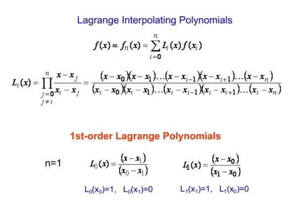
Lagrange Polynomial See http://mathworld.wolfram.com/LagrangeInterpolatingPolynomial.html for more details
Lagrange Polynomial Written explicitly term by term is:
Lagrange Polynomial Results are not always good for animation
Polynomial curve formation • Given by the equation P(u) = au3 + bu2 + cu+ d • u is a parameter that varies from 0 to 1 • u = 0 is the first point on the curve • u = 1 is the last point on the curve • Remember this is a parametric equation! • a, b, c, and d are not scalar values, but vectors
Polynomial curve formation P(u) = au3 + bu2 + cu+ d • The point P(u) = (x(u), y(u), z(u)) where x(u) = axu3 + bxu2 + cxu + dx y(u) = ayu3+ byu2+ cyu+ dy z(u) = azu3+ bzu2+ czu+ dz
Polynomial Curve Formulation Matrix multiplication The point at “time” u Geometric information (i.e the points or tangents) Where u is a scalar value in [0,1] Coefficient matrix (given by which type of curve you are using)
Catmull-Rom spline • Passes through control points • Tangent at each point pi is based on the previous and next points: (pi+1− pi−1) • Not properly defined at start and end • Use a toroidal mapping • Duplicate the first and last points
Catmull-Rom spline derivation τ is a parameter for tension (most implementations set it to 0.5)
Catmull-Rom spline derivation • Use with cubic equation Note: - c values correspond to a, b, c, and d in the earlier cubic equation - c values are vectors
Catmull-Rom spline derivation • Solve for ci in terms of control points
Catmull-Rom matrix form • Set τ to 0.5 and put into matrix form
Blended Parabolas/Catmull-Rom* Visual example * End conditions are handled differently (or assume curve starts at P1 and stops at Pn-2)
Bezier Curve p1 • Find the point x on the curve as a function of parameter u: • x(u) p0 p2 p3
de Casteljau Algorithm • Describe the curve as a recursive series of linear interpolations • Intuitive, but not the most efficient form
de Casteljau Algorithm p1 • Cubic Bezier curve has four points(though the algorithm works with any number of points) p0 p2 p3
de Casteljau Algorithm p1 q1 q0 p0 p2 q2 p3 Lerp = linear interpolation
de Casteljau Algorithm q1 r0 q0 r1 q2
de Casteljau Algorithm r0 • x r1
Bezier Curve p1 • x p0 p2 p3
Cubic Bezier Curve runs through Pi and Pi+3with starting tangent PiPi+1 and ending tangent Pi+2Pi+3
Controlling Motion along p=P(u) Step 1. vary u from 0 to 1 create points on the curve p=P(u) But segments may not have equal length Step 2. Reparameterization by arc length u = U(s) where s is distance along the curve Step 3. Speed control for example, ease-in / ease-out s = ease(t) where t is time
Reparameterizing by Arc Length Analytic Forward differencing Supersampling Adaptive approach Numerically Adaptive Gaussian
Reparameterizing by Arc Length - supersample • Calculate a bunch of points at small increments in u • Compute summed linear distances as approximation to arc length • Build table of (parametric value, arc length) pairs • Notes • Often useful to normalize total distance to 1.0 • Often useful to normalize parametric value for multi-segment curve to 1.0
Speed Control distance • Time-distance function • Ease-in Ease-out • Sinusoidal • Cubic polynomial • Constant acceleration • General distance-time functions time